.ipynb .md .pdf

suggest edit

Binder

Contents

3. Linear inverse problems in function spaces

Many of the notions discussed in the finite-dimensional setting can be extended to the infinite-dimensional setting. We will focus in this chapter on inverse problems where \(K\) is a bounded linear operator and \(\mathcal{U}\) and \(\mathcal{V}\) are (infinite-dimensional) function spaces. The contents of this chapter were heavily inspired by the excellent lecture notes from Matthias J. Ehrhardt and Lukas F. Lang.

Let \(K: \mathcal{U} \rightarrow F\) denote the forward operator, with \(\mathcal{U}\) and \(\mathcal{V}\) Banach spaces. The operator is bounded iff there exists a constant \(C \geq 0\) such that

\[\|Ku\|_{\mathcal{F}} \leq C \|u\|_{\mathcal{U}} \quad \forall u \in \mathcal{U}.\]

The smallest such constant is called the operator norm \(\|K\|\). Note that boundedness also implies continuity, i.e. for any \(u,v \in \mathcal{U}\) we have

\[\|Ku - Kv\|_{\mathcal{F}} \leq C \|u - v\|_{\mathcal{U}}.\]

3.1. Well-posedness

We may again wonder whether the equation \(Ku = f\) is well-posed. To formally analyse this we introduce the following notation:

• \(\mathcal{D}(K) = \mathcal{U}\) denotes the domain of \(K\),

• \(\mathcal{R}(K) = \{Ku\,|\,u\in\mathcal{U}\}\) denotes the range of \(K\),

• \(\mathcal{N}(K) = \{u\in\mathcal{U}\, | \, Ku = 0 \}\) denotes the null-space or kernel of \(K\).

When \(f \not\in \mathcal{R}(K)\), a solution obviously doesn’t exist. We can still look for a solution for which \(Ku \approx f\) by solving

(3.1)\[\min_{u\in \mathcal{U}}\|Ku - f\|_{\mathcal{F}}.\]

A solution to (3.1) is a vector \(\widetilde{u} \in \mathcal{U}\) for which

\[\|K\widetilde{u} - f\|_{\mathcal{F}} \leq \|Ku - f\|_{\mathcal{F}}, \quad \forall u \in \mathcal{U}.\]

If such a vector exists we call it the minimum-residual solution. If the null-space of \(K\) is non-empty, we can construct infinitely many such solutions. We call the one with the smallest norm the minimum-norm solution. Note however that we have not yet proven that such a solution exists in general, nor do we have a constructive way of finding it.

3.2. Bounded operators on Hilbert spaces

To study well-posedness of (3.1) and the corresponding minimum-norm problem we will let \(\mathcal{U}\) and \(\mathcal{F}\) be Hilbert spaces. We will return to analyzing variational problems more generally in a later chapter.

---

First, we introduce the adjoint of \(K\), denoted by \(K^*\) in the usual way as satisfying

\[\langle Ku, f \rangle_{\mathcal{F}} = \langle K^*\!f, u \rangle_{\mathcal{U}}\quad \forall u\in\mathcal{U}, \forall f\in\mathcal{F}.\]

We further denote the orthogonal complement of a subspace \(\mathcal{X} \subset \mathcal{U}\) as

\[\mathcal{X}^\perp = \{u\in\mathcal{U} \, | \, \langle u, v \rangle_{\mathcal{U}}=0 \, \forall \, v \in \mathcal{X}\}.\]

If \(\mathcal{X}\) is a closed subspace we have \((\mathcal{X}^\perp)^\perp = \mathcal{X}\) and we have an orthogonal decomposition of \(\mathcal{U}\) given by \(\mathcal{U} = \mathcal{X} \oplus \mathcal{X}^\perp\), meaning that we can express any \(u\in \mathcal{U}\) as \(u = x + x^\perp\) with \(x\in\mathcal{X}\) and \(x^\perp\in\mathcal{X}^\perp\). The orthogonal projection onto \(\mathcal{X}\) is denoted by \(P_{\mathcal{X}}\). We briefly recall a few useful relations

Lemma : Orthogonal projection

Let \(\mathcal{X} \subset \mathcal{U}\) be a closed subspace. The orthogonal projection onto \(\mathcal{X}\) satisfies the following conditions

1. \(P_{\mathcal{X}}\) is self-adjoint,

2. \(\|P_{\mathcal{X}}\| = 1,\)

3. \(I - P_{\mathcal{X}} = P_{\mathcal{X}^\perp},\)

4. \(\|u - P_{\mathcal{X}}u\|_{\mathcal{U}} \leq \|u - v\|_{\mathcal{U}} \, \forall \, v\in\mathcal{X}\),

5. \(v = P_{\mathcal{X}}u\) iff \(v\in\mathcal{X}\) and \(u-v\in\mathcal{X}^\perp\).

When \(\mathcal{X}\) is not closed we have \((\mathcal{X}^\perp)^\perp = \overline{\mathcal{X}}\) (the closure of \(\mathcal{X}\)). Note that the orthogonal complement of a subspace is always closed.

We now have the following useful relations

• \(\mathcal{R}(K)^\perp = \mathcal{N}(K^*),\)

• \(\mathcal{N}(K^*)^\perp = \overline{\mathcal{R}(K)},\)

• \(\mathcal{R}(K^*)^\perp = \mathcal{N}(K),\)

• \(\mathcal{N}(K)^\perp = \overline{\mathcal{R}(K^*)},\)

from which we conclude that we can decompose \(\mathcal{U}\) and \(\mathcal{F}\) as

• \(\mathcal{U} = \mathcal{N}(K) \oplus \overline{\mathcal{R}(K^*)},\)

• \(\mathcal{F} = \mathcal{N}(K^*) \oplus \overline{\mathcal{R}(K)}.\)

---

We now have the following results

Theorem: Existence and uniqueness of the minimum-residual, minimum-norm solution

Given a bounded linear operator \(K\) and \(f \in \mathcal{F}\), a solution \(\widetilde{u}\) to (3.1)

• only exists if \(f \in \mathcal{R}(K) \oplus \mathcal{R}(K)^\perp\)

• obeys the normal equations \(K^*\! K\widetilde{u} = K^*\! f.\)

The unique solution \(\widetilde{u} \in \mathcal{N}(K)^{\perp}\) to the normal equations is called the minimum-norm solution.

Proof

First, we show that a minimum-residual solution necessarily obeys the normal equations:

• Given a solution \(\widetilde{u}\) to (3.1) and an arbritary \(v\in\mathcal{U}\), define \(\phi(\alpha) = \|K(\widetilde{u} + \alpha v) - f\|_{\mathcal{F}}\). A necessary condition for \(\widetilde{u}\) to be a least-squares solution is \(\phi'(0) = 0\), which gives \(\langle K^*(K\widetilde{u}-f),v \rangle_{\mathcal{U}}\). As this should hold for arbritary \(v\), we find the normal equations. Note that this also implies that \(K\widetilde{u} - f \in \mathcal{R}(K)^\perp\).

Next, we show that the normal equations only allow a solution when \(f \in \mathcal{R}(K)^\perp \oplus \mathcal{R}(K)\).

• Given a solution \(\widetilde{u}\), we find that \(f = K\widetilde{u} + g\) with \(g\in\mathcal{R}(K)^\perp\). Hence, \(f \in \mathcal{R}(K) \oplus \mathcal{R}(K)^\perp\). Conversely, given \(f \in \mathcal{R}(K) \oplus \mathcal{R}(K)^\perp\) , there exist \(u \in \mathcal{U}\) and \(g \in \mathcal{R}(K)^\perp = \left(\overline{\mathcal{R}(K)}\right)^\perp\) such that \(f = Ku + g\). Thus, \(P_{\overline{\mathcal{R}(K)}}f = Ku\). Such a \(u \in \mathcal{U}\) must necessarily be a solution to (3.1) because we have \(\|Ku - f\|_{\mathcal{F}} = \|P_{\overline{\mathcal{R}(K)}}f - f\|_{\mathcal{F}} \leq \inf_{g\in \overline{\mathcal{R}(K)}}\|g - f\|_{\mathcal{F}} \leq \inf_{v\in\mathcal{U}}\|Kv - f\|_{\mathcal{F}}.\) Here, we used the fact that the orthogonal projection on a subspace gives the element closest to the projected element and \(\mathcal{R}(K) \subseteq \overline{\mathcal{R}(K)}\) allows to conclude the last inequality.

Finally, we show that the minimum-norm solution is unique. Denote the minimun-norm solution by \(\widetilde{u}\). Now suppose we have another solution, \(\widetilde{v}\), to (3.1). Since they both solve the normal equations we have \(\widetilde{v} = \widetilde{u} + z\) with \(z \in \mathcal{N}(K)\). It follows that \(\|\widetilde{v}\|_{\mathcal{U}}^2 = \|\widetilde{u}\|_{\mathcal{U}}^2 + 2\langle \widetilde{u}, z \rangle_{\mathcal{U}} + \|z\|_{\mathcal{U}}^2\). Since \(\widetilde{u} \in \mathcal{N}(K)^\perp\) we have \(\langle \widetilde{u}, z \rangle_{\mathcal{U}} = 0\) and hence \(\|\widetilde{v}\|_{\mathcal{U}} \geq \|\widetilde{u}\|_{\mathcal{U}}\) with equality only obtained when \(z = 0\).

---

The Moore-Penrose pseudo-inverse of \(K\) gives us a way to construct the minimum-norm solution defined above. We can think of this pseudo-inverse as the inverse of a restricted forward operator.

Definition: Moore-Penrose inverse

Given an bounded linear operator \(K:\mathcal{U}\rightarrow \mathcal{F}\) we denote its restriction to \(\mathcal{N}(K)^\perp\) as \(\widetilde{K}:\mathcal{N}(K)^\perp\rightarrow\mathcal{R}(K)\). The M-P inverse \(K^\dagger: \mathcal{R}(K)\oplus\mathcal{R}(K)^\perp \rightarrow \mathcal{N}(K)^\perp\) is defined as the unique linear extension of \(\widetilde{K}^{-1}\) with \(\mathcal{N}(K^\dagger) = \mathcal{R}(K)^\perp\).

The range of \(K^\dagger\)

Let \(u\in\mathcal{R}(K^\dagger)\), then there exists a \(f\in\mathcal{D}(K^\dagger)\) such that \(u = K^\dagger f\). By definition we can decompose \(f = f_1 + f_2\) with \(f_1\in\mathcal{R}(K)\), \(f_2 \in \mathcal{R}(K)^\perp\). Thus \(K^\dagger f = K^\dagger f_1 = \widetilde{K}^{-1}f_1\). Hence, \(u \in \mathcal{R}(\widetilde{K}^{-1}) = \mathcal{N}(K)^\perp\). This establishes that \(\mathcal{R}(K^\dagger)\subseteq \mathcal{N}(K)^\perp\). Conversely, let \(u\in\mathcal{N}(K)^\perp\). Then \(u = \widetilde{K}^{-1}\widetilde{K} = K^\dagger K u\), whence \(\mathcal{N}(K)^\perp \subseteq \mathcal{R}(K^\dagger)\). We conclude that \(\mathcal{R}(K^\dagger) = \mathcal{N}(K)^\perp\).

The pseudo-inverse satisfies a few useful relations:

Theorem: Moore-Penrose equations

The M-P pseudo-inverse \(K^{\dagger}: \mathcal{R}(K)^\perp \oplus \mathcal{R}(K) \rightarrow \mathcal{N}(K)^\perp\) of \(K\) is unique and obeys the following useful relations:

1. \(KK^\dagger = \left.P_{\overline{\mathcal{R}(K)}}\right|_{\mathcal{D}(K^\dagger)}.\)

2. \(K^\dagger K = I - P_{\mathcal{N}(K)},\)

3. \(K^\dagger K K^\dagger = K^\dagger,\)

4. \(KK^\dagger K = K,\)

Proof

1. Decompose \(f \in \mathcal{D}(K^\dagger)\) as \(f = f_1 + f_2\) with \(f_1\in\mathcal{R}(K)\), \(f_2\in\mathcal{R}(K)^\perp\) and use that \(K = \widetilde{K}\) on \(\mathcal{N}(K)^\perp\). Then \(KK^\dagger f = K\widetilde{K}^{-1}f_1 = f_1\). Hence, \(KK^\dagger\) acts as an orthogonal projection of \(f \in \mathcal{D}(K^\dagger)\) on \(\overline{\mathcal{R}(K)}\).

2. Decompose \(u \in \mathcal{U}\) in two parts \(u = u_1 + u_2\) with \(u_1 \in \mathcal{N}(K)\), \(u_2\in\mathcal{N}(K)^\perp\) we have \(K^\dagger K u = K^\dagger K u_1 = u_1\), so \(KK^\dagger\) acts like an orthogonal projection on \(\mathcal{N}(K)^\perp\) so \(KK^\dagger = I - P_{\mathcal{N}(K}\) (note that the orthogonal complement of a subspace is always closed).

3. Since \(KK^\dagger\) projects onto \(\overline{R}(K)\), it filters out any components in \(f\) in the null-space of \(K^\dagger\) which would disappear anyway.

4. Since \(K^\dagger K\) projects on \(\mathcal{N}(K)^\perp\) if filters out any components in the null-space of \(K\), which would disappear anyway.

With these, we can show that the minimum-norm solution to (3.1) is obtained by applying the pseudo-inverse to the data.

Theorem: Minimum-norm solution

Let \(K\) be a bounded linear operator with pseudo-inverse \(K^{\dagger}\) and \(f \in \mathcal{D}(K^\dagger)\), then the unique minimum-norm solution to (3.1) is given by

\[\widetilde{u} = K^\dagger f.\]

Proof

We know that for \(f \in \mathcal{D}(K^\dagger)\) the minimum-norm solution \(\widetilde{u} \in \mathcal{N}(K)^\perp\) exists and unique. Using the fact that \(K\widetilde{u} = P_{\overline{\mathcal{R}(K)}}f\) (due to the \textit{mimimum-residual} solution property) and the M-R equations, we have \(\widetilde{u} = (I - P_{\mathcal{N}}(K))\widetilde{u} = K^\dagger K\widetilde{u} = K^\dagger P_{\overline{\mathcal{R}(K)}}f = K^\dagger K K^\dagger f = K^\dagger f\).

When defining the the solution through the M-P pseudo-inverse, we have existence uniqueness of the minimum-norm to (3.1). However, we cannot expect stability in general. For this, we would need \(K^{\dagger}\) to be continuous. To see this, consider noisy data \(f^{\delta} = f + e\) with \(\|e\|\leq \delta\). For stability of the solution we need to bound the difference between the corresponding solutions \(\widetilde{u}\), \(\widetilde{u}^\delta\):

\[\|\widetilde{u} - \widetilde{u}^\delta\|_{\mathcal{U}} = \|K^{\dagger}e\|_{\mathcal{F}},\]

which we can only do when \(K^\dagger\) is continuous (or, equivalently, bounded).

Theorem: Continuity of the M-P pseudo-inverse

The pseudo-inverse \(K^\dagger\) of \(K\) is continuous iff \(\mathcal{R}(K)\) is closed.

Proof

For the proof, we refer to Thm 2.5 of these lecture notes.

---

Let’s consider a concrete example.

Example: Pseudo-inverse of a bounded operator

Consider the following forward operator

\[Ku(x) = \int_{-\infty}^\infty k(x-y)u(y)\mathrm{d}y,\]

with \(k, u \in L^{1}(\mathbb{R})\). Young’s inequality tells us that \(\|Ku\|_{L^1(\mathbb{R})} \leq \|k\|_{L^1(\mathbb{R})} \cdot \|u\|_{L^1(\mathbb{R})}\) and hence that \(K\) is bounded.

We can alternatively represent \(K\) using convolution theorem as

\[Ku(x) = F^{-1} (\widehat{k} \widehat{u}) (x),\]

where \(F : L^1(\mathbb{R}) \rightarrow L^{\infty}(\mathbb{R})\) denotes the Fourier transform and \(\widehat{k} = Fk\), \(\widehat{u} = Fu\).

This suggests defining the inverse of \(K\) as

\[K^{-1}f = F^{-1} (\widehat{f} / \widehat{k}).\]

We note here that, by the Riemann–Lebesgue lemma, the Fourier transform of \(k\) tends to zero at infinity. This means that the inverse of \(K\) is only well-defined when \(\widehat{f}\) decays faster than \(\widehat{k}\). However, we can expect problems when \(\widehat{k}\) has roots as well.

As a concrete example, consider \(k = \text{sinc}(x)\) with \(\widehat{k}(\xi) = H(\xi+1/2)-H(\xi-1/2)\). The forward operator then bandlimits the input. Can you think of a function in the null-space of \(K\)?

The pseudo-inverse may now be defined as

\[K^{\dagger}f = F^{-1} B \widehat{f},\]

where

\[\begin{split}B\widehat{f}(\xi) = \begin{cases} \widehat{f}(\xi) & |\xi| \leq 1/2 \\ 0 & \text{otherwise}\end{cases}.\end{split}\]

3.3. Compact operators

An important subclass of the Bounded operators are the compact operators. They can be thought of as a natural generalization of matrices to the infinite-dimensional setting. Hence, we can generalize the notions from the finite-dimensional setting to the infinite-dimensional setting.

---

There are a number of equivalent definitions of compact operators. We will use the following.

Definitition: Compact operator

An operator \(K: \mathcal{U} \rightarrow \mathcal{F}\) with \(\mathcal{U},\mathcal{F}\) Hilbert spaces, is called compact if it can be expressed as

\[ K = \sum_{j=1}^{\infty} \sigma_j \langle \cdot, v_j\rangle_{\mathcal{U}}u_j, \]

where \(\{v_i\}\) and \(\{u_i\}\) are orthonormal bases of \(\mathcal{N}(K)^\perp\) and \(\overline{\mathcal{R}(K)}\) respectively and \(\{\sigma_i\}\) is a null-sequence (i.e., \(\lim_{i\rightarrow \infty} \sigma_i = 0\)). We call \(\{(u_i, v_i, \sigma_i)\}_{j=1}^\infty\) the singular system of \(K\). The singular system obeys

\[Kv_j = \sigma_j u_j, \quad K^*u_j = \sigma_j v_j.\]

An important subclass of the compact operators are the Hilbert-Schmidt integral operators, which can be written as

\[Ku(x) = \int_{\Omega} k(x,y) u(y) \mathrm{d}y,\]

where \(k: \Omega \times \Omega \rightarrow \mathbb{R}\) is a Hilbert-Schmidt kernel obeying \(\|k\|_{L^2(\Omega\times\Omega)} < \infty\) (i.e., it is square-integrable).

---

The pseudo-inverse of a compact operator is defined analogously to the finite-dimensional setting:

Definition: Pseudo-inverse of a compact operator

The pseudo-inverse of a compact operator \(K: \mathcal{U} \rightarrow \mathcal{F}\) is expressed as

\[ K^{\dagger} = \sum_{j=1}^{\infty} \sigma_j^{-1} \langle \cdot, u_j\rangle_{\mathcal{F}}v_j, \]

where \(\{(u_i, v_i, \sigma_i)\}_{i=1}^\infty\) is the singular system of \(K\)

With this we can precisely state the Picard condition.

Definition: Picard condition

Given a compact operator \(K: \mathcal{U} \rightarrow \mathcal{F}\) and \(f \in \mathcal{F}\), we have that \(f \in \mathcal{R}(K) \cup \mathcal{R}(K)^\perp\) iff

(3.2)\[\sum_{j=1}^{\infty} \frac{|\langle f, u_j\rangle_{\mathcal{F}}|^2}{\sigma_j^2} < \infty.\]

Remark : Degree of ill-posedness

For inverse problems with compact operators we can thus use the Picard condition to check if (3.1) has a solution. Although this establishes existence and uniqueness through the pseudo-inverse, it does not guarantee stability as \(\sigma_j \rightarrow 0\). If \(\sigma_j\) decays exponentially, we call the problem severely ill-posed, otherwise we call it mildly ill-posed.

---

Let’s consider a few examples.

Example: A sequence operator

Consider the operator \(K:\ell^2 \rightarrow \ell^2\), given by

\[ u = (u_1,u_2,...) \mapsto (0,u_2,\textstyle{\frac{1}{2}}u_3,...), \]

i.e. we have an infinite matrix operator of the form

\[\begin{split} K = \left(\begin{matrix} 0 & & & & \\ & 1 & & & \\ & & \frac{1}{2} & & \\ & & & \ddots & \\ \end{matrix}\right) \end{split}\]

The operator is obviously linear. To show that is bounded we’ll compute its norm:

\[ \|K\| = \sup_{u \neq 0} \frac{\|Ku\|_{\ell^2}}{\|u\|_{\ell^2}} = 1. \]

derivation

We can fix \(\|u\|_{\ell_2} = 1\) and verify that the maximum is obtained for \(u = (0,1,0,\ldots)\) leading to \(\|K\| = 1\).

To show that the operator is compact, we explicitly construct its singular system, giving: \(u_i = v_i = e_i\) with \(e_i\) the \(i^{\text{th}}\) canonical basis vector and \(\sigma_1 = 0\), \(\sigma_{i} = (i-1)^{-1}\) for \(i > 1\).

derivation

Indeed, it is easily verified that \(Ke_i = \sigma_i e_i\).

The pseudo inverse is then defined as

\[\begin{split} K^{\dagger} = \left(\begin{matrix} 0 & & & & \\ & 1 & & & \\ & & 2 & & \\ & & & \ddots & \\ \end{matrix}\right) \end{split}\]

This immediately shows that \(K^\dagger\) is not bounded. Now consider obtaining a solution for \(f = (1,1,\textstyle{\frac{1}{2}}, \textstyle{\frac{1}{3}},\ldots)\). Applying the pseudo-inverse would yield \(K^\dagger f = (0,1, 1, \ldots)\) which is not in \(\ell_2\). Indeed, we can show that \(f \not\in \mathcal{R}(K) \oplus \mathcal{R}(K)^\perp\). The problem here is that the range of \(K\) is not closed.

---

Example: Differentiation

Consider \(K:L_2([0,1]) \rightarrow L_2([0,1])\) defined as

\[ Ku(x) = \int_0^x u(y)\mathrm{d}y. \]

Given \(f(x) = Ku(x)\) we would naively let \(u(x) = f'(x)\). Let’s analyse this in more detail.

The operator can be expressed as

\[ Ku(x) = \int_0^1 k(x,y)u(y)\mathrm{d}y, \]

with \(k(x,y) = H(x-y)\), where \(H\) denotes the Heaviside stepfunction. The operator is compact because \(k\) is square integrable.

derivation

Indeed, we have

\[\int_0^1 \int_0^1 |k(x,y)|^2 \mathrm{d}x\mathrm{d}y = \textstyle{\frac{1}{2}}.\]

We conclude that \(k\) is a Hilbert-Schmidt kernel and hence that \(K\) is compact.

The adjoint is found to be

\[ K^*f(y) = \int_0^1 k(x,y) f(x)\mathrm{d}x = \int_y^1 f(x)\mathrm{d}x. \]

derivation

Using the definition we find

\[K^*f(y) = \int_0^1 k(x,y)f(x)\mathrm{d}x = \int_y^1 f(x)\mathrm{d}x.\]

The singular system is given by

\[ \sigma_k = ((k+1/2)\pi)^{-1}, \]

\[ u_k(x) = \sqrt{2}\sin(\sigma_k^{-1} x), \]

\[ \quad v_k(x) = \sqrt{2}\cos(\sigma_k^{-1} x). \]

derivation

To derive the singular system, we first need to compute the eigenpairs \((\lambda_k, v_k)\) of \(K^*K\). The singular system is then given by \((\sqrt{\lambda_k}, (\sqrt{\lambda_k})^{-1}Kv_k, v_k)\).

We find

\[ K^*Kv(y) = \int_y^1 \int_0^x v(z) \, \mathrm{d}z\mathrm{d}x = \lambda v(y). \]

At \(y = 1\) this yields \(v(1) = 0\). Differentiating, we find

\[ \lambda v'(y) = -\int_0^y v(z)\mathrm{d}z, \]

which yields \(v'(0) = 0\). Differentiating once again, we find

\[ \lambda v''(x) = -v(x). \]

The general solution to this differential equation is

\[ v(x) = a\sin(x/\sqrt{\lambda}) + b\cos(x/\sqrt{\lambda}). \]

Using the boundary condition at \(x = 0\) we find that \(a = 0\). Using the boundary condition at \(x = 1\) we get

\[ b\cos(1/\sqrt{\lambda}) = 0, \]

which yields \(\lambda_k = 1/((k + 1/2)^2\pi^2)\), \(k = 0, 1, \ldots\). We choose \(b\) to normalize \(\|v_k\| = 1\).

The operator can thus be expressed as

\[ Ku(x) = \sum_{k=0}^\infty \frac{\langle u, v_k\rangle}{(k+1/2)\pi} u_k(x), \]

and the pseudo-inverse by

\[ K^{\dagger}f(x) = \pi\sum_{k=0}^\infty (k+1/2)\langle f, u_k\rangle v_k(x). \]

We can now study the ill-posedness of the problem by looking at the Picard condition

\[ \|K^\dagger f\|^2 = \pi^2\sum_{k=0}^\infty f_k^2 (k+1/2)^2, \]

where \(f_k = \langle f, u_k\rangle\) are the (generalized) Fourier coefficients of \(f\).

For this infinite sum to converge, we need strong requirements on \(f_k\); for example \(f_k = 1/k\) does not suffice to make the sum converge. This is quite surprising since such an \(f\) is square-integrable. It turns out we need \(f_k = \mathcal{O}(1/k^2)\) to satisfy the Picard condition. Effectively this means that \(f'\) needs to be square integrable. This makes sense since we saw earlier that \(u(x) = f'(x)\) is the solution to \(Ku = f\).

3.4. Regularization

3.4.1. Truncation and Tikhonov regularization

In the previous section we saw that the pseudo-inverse of a compact operator is not bounded (continuous) in general. To counter this, we introduce the regularized pseudo-inverse:

\[ K_{\alpha}^{\dagger}f = \sum_{k=0}^{\infty} g_{\alpha}(\sigma_k) \langle f, u_k\rangle v_k, \]

where \(g_{\alpha}\) determines the type of regularization used. For Tikhonov regularisation we let

\[ g_{\alpha}(s) = \frac{s}{s^2 + \alpha}= \frac{1}{s + \alpha/s}. \]

For a truncated SVD we let

\[\begin{split} g_{\alpha}(s) = \begin{cases} s^{-1} & \text{if}\, s > \alpha \\ 0 & \text{otherwise} \end{cases}. \end{split}\]

We can show that the regularized pseudo inverse, \(K_{\alpha}^{\dagger}\), is bounded for \(\alpha > 0\) and converges to \(K^\dagger\) as \(\alpha \rightarrow 0\).

Given noisy data \(f^{\delta} = f + e\) with \(\|e\| \leq \delta\), we can now study the effect of regularization by studying the error. The total error is now given by

\[ \|K_{\alpha}^\dagger f^\delta - K^\dagger f\|_{\mathcal{U}} \leq \|K_{\alpha}^\dagger f - K^\dagger f\|_{\mathcal{U}} + \|K_{\alpha}^\dagger(f^\delta - f)\|_{\mathcal{U}}, \]

in which we recognize the bias and variance contributions. Note that we may bound this even further as

\[\|K_{\alpha}^\dagger f^\delta - K^\dagger f\|_{\mathcal{U}} \leq \|K_{\alpha}^\dagger - K^\dagger\| \|f\|_{\mathcal{F}} + \delta \|K_{\alpha}^\dagger\|.\]

Alternatively, we may express the error in terms of the minimum-norm solution \(u = K^{\dagger} Ku = K^\dagger f\) as

\[\|K_{\alpha}^\dagger f^\delta - K^\dagger f\|_{\mathcal{U}} \leq \|I - K_{\alpha}^\dagger K\| \|u\|_{\mathcal{U}} + \delta \|K_{\alpha}^\dagger\|.\]

Such upper bounds may be useful to study asymptotic properties of the problem but may be too loose to be used in practice. In that case a more detailed analysis incorporating the type of noise and the class of images \(u\) that we are interested in is needed.

Example: Differentiation

Consider adding Tikhonov regularisation to stabilise the differentiation problem. Take measurements \(f^{\delta} = Ku + \delta\sin(\delta^{-1}x)\), where \(\delta = \sigma_k\) for some \(k\). The error \(K^\dagger f^{\delta} - u\) is then given by

\[ K^\dagger K u - u + \delta K^{\dagger}\sin(\delta^{-1}\cdot). \]

Because \(\delta^{-1} = \sigma_k\) and \(\sin(\sigma_k^{-1}x)\) is a singular vector of \(K\) (or because the pseudo-inverse acts as taking a derivative), this simplifies to

\[ \cos(\sigma_k^{-1}x). \]

Thus, the reconstruction error does not go to zero as \(\delta\downarrow 0\), even though the error in the data does.

The eigenvalues of \(K_{\alpha}^\dagger K\) are given by \((1 + \alpha \sigma_k^{-2})^{-1}\), with \(\sigma_k = (\pi(k + 1/2))^{-1}\). The bias is thus given by

\[ \|I - K_{\alpha}^\dagger K\| = \max_{k} \left|1 - (1 + \alpha \sigma_{k}^{-2})^{-1}\right|. \]

Likewise, the variance is given by

\[ \|K_{\alpha}^\dagger\| = \max_{k}\frac{1}{\sigma_k + \alpha \sigma_{k}^{-1}}. \]

3.4.2. Generalized Tikhonov regularization

We have seen in the finite-dimensional setting that Tikhonov regularization may be defined through a variational problem:

\[ \min_{u} \|Ku - f\|^2_{\mathcal{F}} + \alpha \|u\|^2_{\mathcal{U}}. \]

It turns out we can do the same in the infinite-dimensional setting. Indeed, we can show that the corresponding normal equations are given by

\[(K^*\!K + \alpha I)u = K^*f.\]

Generalized Tikhonov regularization is defined in a similar manner through the variation problem

\[ \min_{u} \|Ku - f\|^2_{\mathcal{F}} + \alpha \|Lu\|^2_{\mathcal{V}}, \]

where \(L:\mathcal{U}\rightarrow \mathcal{V}\) is a (not necessarily bounded) linear operator. The corresponding normal equations can be shown to be

\[(K^*\!K + \alpha L^*\!L)u = K^*f.\]

We can expect a unique solution when the intersection of the kernels of \(K\) and \(L\) is empty. In many applications, \(L\) is a differential operator. This can be used to impose smoothness on the solution.

3.4.3. Parameter-choice strategies

Given a regularization strategy with parameter \(\alpha\), we need to pick \(\alpha\). As mentioned earlier, we need to pick \(\alpha\) to optimally balance between the bias and variance in the error. To highlight the basic flavors of parameter-choice strategies, we give three examples.

Example: A-priori rules

Assuming that we know the noise level \(\delta\), we can define a parameter-choice rule \(\alpha(\delta)\). We call such a rule convergent iff

\[\lim_{\delta\rightarrow 0} \alpha(\delta) = 0, \quad \lim_{\delta\rightarrow 0} \delta \|K_{\alpha(\delta)}^\dagger\| = 0.\]

With these requirements, we can easily show that the error \(\|K_{\alpha}^\dagger f^{\delta} - K^\dagger f\|_{\mathcal{U}} \rightarrow 0\) as \(\delta\rightarrow 0\).

Such parameter-choice rules are nice in theory, but hard to design in practice. One is sometimes interested in the convergence rate, which aims to bound the bias in terms of \(\delta^\nu\) for some \(0 < \nu < 1\).

Example: The discrepancy principle

Morozov’s discrepancy principle chooses \(\alpha\) such that

\[\|KK_{\alpha}^\dagger f^{\delta} - f^{\delta}\|_{\mathcal{F}} \leq \eta \delta,\]

with \(\eta > 1\) a fixed parameter. This can be interpreted as finding an \(\alpha\) for which the solution fits the data in accordance with the noise level. Note, however, that such an \(\alpha\) may not exist if (a significant part of) \(f^\delta\) lies in the kernel of \(K^*\). This is an example of an a-posterior parameter selection rule, as it depends on both \(\delta\) and \(f^\delta\).

Example: The L-curve method

Here, we choose \(\alpha\) via

\[\min_{\alpha > 0} \|K_{\alpha}^\dagger f^\delta\|_{\mathcal{U}} \|KK_{\alpha}^\dagger f^\delta - f^\delta\|_{\mathcal{F}}.\]

The name stems from the fact that the optimal \(\alpha\) typically resides at the corner of the curve \((\|K_{\alpha}^\dagger f^\delta\|_{\mathcal{U}}, \|KK_{\alpha}^\dagger f^\delta - f^\delta\|_{\mathcal{F}})\).

This rule has the practical advantage that no knowledge of the noise level is required. Such a rule is called a heuristic method. Unfortunately, it is not a convergent rule.

3.5. Exercises

3.5.1. Convolution

Consider the example in section 3.2 with \(k(x) = \exp(-|x|)\).

• Is the inverse problem ill-posed?

• For which functions \(f\) is the inverse well-defined?

Answer

Here we have \(\widehat{k}(\xi) = \sqrt{2/\pi} (1 + \xi^2)^{-1}\) (cf. this table). For the inverse we then need \((1 + \xi^2)\widehat{f}(\xi)\) to be bounded. We conclude that the inverse problem is ill-posed since a solution will not exist for all \(f\). Moreover, we can expect amplification of the noise if it has non-zero Fourier coefficients for large \(|\xi|\).

We can only define the inverse for functions \(f\) whose Fourier transform decays rapidly in the sense that \(\lim_{|\xi|\rightarrow} (1 + \xi^2)\widehat{f}(\xi) < \infty\). Examples are \(f(x) = e^{-ax^2}\) or \(f(x) = \text{sinc}(ax)\) for any \(a > 0\). We may formalise this by introducing Schwartz functions but this is beyond the scope of this course.

3.5.2. Differentiation

Consider the forward operator

\[ Ku(x) = \int_0^x u(y)\mathrm{d}y. \]

We’ve seen in the example that the inverse problem is ill-posed. Consider the regularized least-squares problem

\[\min_{u} \|Ku - f^\delta\|^2 + \alpha \|u'\|^2,\]

with \(\|\cdot\|\) denoting the \(L^2([0,1])\)-norm. In this exercise we are going to analyze how this type of regularization addresses the ill-posedness by looking at the variance term.

• Show that the corresponding regularized pseudo-inverse is given by

\[K_{\alpha}^\dagger = \sum_{k=0}^\infty \frac{\sigma_k \langle u_k, \cdot \rangle}{\sigma_k^2 + \alpha \sigma_k^{-2}} v_k(x),\]

where \(\{(u_k,v_k,\sigma_k)\}_{k=0}^\infty\) denotes the singular system of \(K\).

• Take \(f^\delta(x) = f(x) + \sigma_k \sqrt{2}\sin(\sigma_k^{-1}x)\) with \(\sigma_k\) a singular value of \(K\) and show that for \(\alpha > 0\) the variance \(\|K_{\alpha}^\dagger (f^\delta - f)\| \rightarrow 0\) as \(k \rightarrow 0\)

Answer

We will use the SVD of \(K\) to express the solution and derive a least-squares problem for the coefficients of \(u\) using the orthonormality of the singular vectors.

The right singular vectors are given by \(v_k(x) = \sqrt{2}\cos\left(\sigma_k^{-1} x\right)\) with \(\sigma_k = (\pi(k+1/2))^{-1}\). Since these constitute an orthonormal basis for the orthogonal complement of the kernel of \(K\) we can express \(u\) as

\[u(x) = \sum_{k=0}^\infty a_k v_k(x) + w, \]

with \(Kw = 0\). We’ll ignore \(w\) for the time being and assume without proof that \(\{v_k\}_{k=0}^\infty\) is an orthonormal basis for \(L^2([0,1])\).

We can now express the least-squares problem in terms of the coefficients \(a_k\) First note that

\[u'(x) = -\sum_{k=0}^\infty \sigma_k^{-1}a_k u_k(x),\]

with \(u_k(x)\) denoting the left singular vectors \(u_k(x) = \sqrt{2}\sin\left(\sigma_k^{-1} x\right)\). Then

\[\|u'\|^2 = \sum_{k=0}^\infty \frac{a_k^2}{\sigma_k^2},\]

and using the fact that \(Kv_k = \sigma_k u_k\):

\[\|Ku - f\|^2 = \sum_{k=0}^\infty (\sigma_k a_k - f_k)^2,\]

with \(f_k = \langle u_k, f\rangle\). The normal equations are now given by

\[\left(\sigma_k^2 + \alpha \sigma_k^{-2}\right)a_k = \sigma_k f_k,\]

yielding

\[u(x) = \sum_{k=0}^\infty \frac{\sigma_k \langle u_k, f \rangle}{\sigma_k^2 + \alpha \sigma_k^{-2}} v_k(x).\]

We can now study what happens to the variance term \(\|K_{\alpha}^\dagger e\|\) with \(e_k(x) = \sigma_k \sin(x/\sigma_k)\). First note that (by orthogonality)

\[K_{\alpha}^\dagger e_k(x) = \frac{\sigma_k^2}{\sigma_k^2 + \alpha \sigma_k^{-2}} \cos(\sigma_k^{-1} x).\]

We see, as before, that for \(\alpha = 0\) the variance is constant as \(k\rightarrow \infty\) (i.e, noise level going to zero). For \(\alpha > 0\), however, we see that the variance tends to zero.

3.5.3. Convergent regularization

Consider the regularized pseudo-inverse

\[K^\dagger_{\alpha} = \sum_{k=0}^\infty g_{\alpha}(\sigma_k) \langle u_k,\cdot\rangle v_k,\]

and let \(f^\delta = f + e\) with \(\|e\|_{\mathcal{F}} \leq \delta\). We are going to study the convergence of this method, i.e., how fast \(\|K_{\alpha}^\dagger f^\delta - K^\dagger f\| \rightarrow 0\). You may assume that \(f \in \mathcal{R}(K)\) and that \(f^\delta\) obeys the Picard condition. We further let

\[\begin{split}g_{\alpha}(s) = \begin{cases} s^{-1} & s > \alpha \\ 0 & s \leq \alpha \end{cases}.\end{split}\]

and \(\alpha(\delta) = \sqrt{\delta}\).

• Show that the total error \(\|K_{\alpha}^\dagger f^\delta - K^\dagger f\|\) converges to zero as \(\delta \rightarrow 0\).

• Show that the variance term converges to zero as \(\delta\rightarrow 0\) with rate \(1/2\):

\[\|K_{\alpha}^\dagger e\|_{\mathcal{U}} = \mathcal{O}(\sqrt{\delta}).\]

Under additional assumptions on the minimum-norm solution we can provide a faster convergence rate in. Assume that for a given \(\mu > 0\) there exists a \(w\) such that \(K^\dagger f = (K^*K)^{\mu} w\).

• Show that this condition implies that (i.e., more regularity of \(f\))

\[\sum_{k=0}^{\infty} \frac{|\langle f,u_k\rangle|^2}{\sigma_k^{2(1 + 2\mu)}} < \infty.\]

• Show that

\[\|K^\dagger_{\alpha} f - K^\dagger f\| = \mathcal{O}(\delta^{\mu}).\]

Answer

• We split the error in its bias and variance terms and consider each separately. The bias term is given by \(\|(K^\dagger - K_{\alpha}^\dagger)f\|\), which we express as

\[\|(K^\dagger - K_{\alpha}^\dagger)f\|^2 = \sum_{k=0}^\infty (\sigma_k^{-1} - g_{\alpha}(\sigma_k))^2 |\langle f, u_k\rangle|^2.\]

We can split off a factor \(\sigma_k^{-1}\) and bound as

\[\|(K^\dagger - K_{\alpha}^\dagger)f\|^2 \leq \sup_k (1 - \sigma_k g_{\alpha}(\sigma_k))^2 \sum_{k=0}^\infty \frac{|\langle f, u_k\rangle|^2}{\sigma_k^2}.\]

Since \(f\) obeys the Picard condition, the second term is finite. The first term can be bounded because \(0 < sg_{\alpha}(s) \leq 1\). Moreover, we see that at \(\alpha = 0\) we have \((1 - \sigma_k g_{\alpha}(\sigma_k))^2 = 0\). We conclude that the bias converges to zero as \(\delta \rightarrow 0\). We do not get a rate, however.

The variance term can be shown to converge to zero as well, as done below.

• We find

\[\|K^\dagger_{\alpha} e\| \leq \|K^\dagger_{\alpha}\| \delta,\]

with \(\|K^\dagger_{\alpha(\delta)}\| = \sup_k |g_{\alpha(\delta)}(\sigma_k)|\). To bound this, we observe that \(|g_{\alpha}(s)| \leq \alpha^{-1}\). Setting \(\alpha = \sqrt{\delta}\) we get the desired result.

• Start from

\[\sum_{k=0}^{\infty} \frac{|\langle f,u_k\rangle|^2}{\sigma_k^{2 + 4\mu}}\]

and substitute \(f = K(K^*K)^{\mu} w = \sum_{k=0}^\infty \sigma_k^{2\mu+1}\langle w,u_k\rangle u_k\) to get

\[\sum_{k=0}^{\infty} \sigma_k^{2 + 4\mu}\frac{|\langle w,u_k\rangle|^2}{\sigma_k^{2 + 4\mu}} = \|w\|^2 < \infty.\]

• Starting again from the bias term, we can factor out an additional \(\sigma^{4\mu}\) term. We then use that \(s^{2\mu}(1 - sg_{\alpha}(s)) \leq \alpha^{2\mu} \) to find the desired result.

3.5.4. Convolution through the heat equation

In this exercise we’ll explore the relation between the heat equation and convolution with a Gaussian kernel. Define the forward problem \(f = Ku\) via the initial-value problem

\[ v_t = v_{xx}, \quad v(0,x) = u(x), \quad f(x) = v(T,x). \]

• Verify that the solution to the heat equation is given by

\[ v(t,x) = \int_{\mathbb{R}} u(x') g_t(x - x')\mathrm{d}x', \]

where \(g_t(x)\) is the heat-kernel:

\[ g_t(x) = \frac{1}{2\sqrt{\pi t}}\exp(-(x/2)^2/t). \]

You may assume that \(u\) is sufficiently regular and use that \(g_t(x)\) converges (in the sense of distributions) to \(\delta(x)\) as \(t \downarrow 0\).

• Show that we can thus express the forward operator as

\[ Ku(x) = \frac{1}{2\sqrt{\pi T}}\int_{\mathbb{R}} u(x') \exp(-(x - x')^2/(4T)) \mathrm{d}x'. \]

• Show that the operator may be expressed as

\[ Ku = F^{-1}((Fu)\cdot(Fg_T)), \]

where \(\cdot\) denotes point-wise multiplication and \(F\) denotes the Fourier transform.

• Express the inverse of \(K\) as multiplication with a filter \(\widehat{h}\) (in the Fourier domain). How does ill-posed manifest itself here and how does it depend on \(T\) ?

We define a regularized filter (in the Fourier domain) by band limitation:

\[\begin{split}\widehat{h}_{\alpha}(\xi) = \begin{cases} \widehat{h}(\xi) & \text{for} & |\xi|\leq \alpha^{-1} \\ 0 & \text{for} &|\xi| > \alpha^{-1}\end{cases}.\end{split}\]

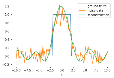
• Test its effect numerically on noisy data for \(T = 2\) using the code below. In particular, design an a-priori parameter selection rule \(\alpha(\delta)\) that ensures that the total error converges and stays below 1 (in relative sense). Does this rule do better than the naive choice \(\alpha(\delta) = \delta\)?

import numpy as np
import matplotlib.pyplot as plt

# grid and parameters
T = 10
delta = 1e-1
alpha = 20
n = 100
x = np.linspace(-10,10,n)
xi = np.fft.rfftfreq(n, d=1.0)

# define ground truth
u = np.heaviside(2-np.abs(x),1)

# define operator
gh = np.exp(-T*(2*np.pi*xi)**2)
K = lambda u : np.fft.irfft(np.fft.rfft(u)*gh)

# define regularised inverse
w = lambda alpha : np.piecewise(xi, [np.abs(xi) <= 1/alpha, np.abs(xi) > 1/alpha], [1, 0])
R = lambda alpha,f : np.fft.irfft(w(alpha)*np.fft.rfft(f)/gh)

# generate noisy data
f_delta = K(u) + delta*np.random.randn(n)

# reconstruction
u_alpha_delta = R(alpha,f_delta)

# plot
plt.plot(x,u,label='ground truth')
plt.plot(x,f_delta,label='noisy data')
plt.plot(x,u_alpha_delta,label='reconstruction')
plt.xlabel(r'$x$')
plt.legend()
plt.show()

Answer

• We can easily verify that it indeed satisfies the differential equation by computing \(v_t\) and \(v_{xx}\). To show that it satisfies the initial condition, we take the limit \(t\rightarrow 0\) and use that \(\lim_{t\rightarrow 0} \int g_t(x)u(x) \mathrm{d}x = u(0)\).

• Setting \(t = T\) in the previous expression gives the desired result.

• This follows from the convolution theorem.

• The inverse of \(K\) is naively given by multiplication with \((Fg_T)^{-1}\) in the Fourier domain. We have \(\widehat{g}_T(\xi) \propto e^{-T \xi^2}\) so we can only usefully define the inverse on functions whose Fourier spectrum decays fast enough such that the inverse Fourier transform of \(\widehat{f}/\widehat{g}_T\) can be defined. Thus a solution does not exist for a large class of \(f\) and noise is amplified exponentially. This only gets worse for larger \(T\).

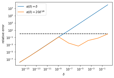
• See the code below. We compute the total error using the function reconstruct which computes noisy data and reconstructs using the regularised inverse. To get a more stable result we average over a number of random instances of the noise. Using \(\alpha(\delta) = \delta\) gives a (numerically) convergent result, however for large \(\delta\) it gives a very large error. Picking \(\alpha(\delta)\) to converge a bit slower allows one to keep the relative total error below 1. Note that we only show convergence of the error for one particular \(u\), so we cannot conclude that this will work in general as in a previous exercise. If you like Fourier analysis and sampling theory, this may be a nice exercise.

import numpy as np
import matplotlib.pyplot as plt

# grid and parameters
T = 2
delta = 1e-1
alpha = 20
n = 100
x = np.linspace(-10,10,n)
xi = np.fft.rfftfreq(n, d=1.0)

# define ground truth
u = np.heaviside(2-np.abs(x),1)

# define operator
gh = np.exp(-T*(2*np.pi*xi)**2)
K = lambda u : np.fft.irfft(np.fft.rfft(u)*gh)

# define regularised inverse
w = lambda alpha : np.piecewise(xi, [alpha*np.abs(xi) <= 1, alpha*np.abs(xi) > 1], [1, 0])
R = lambda alpha,f : np.fft.irfft(w(alpha)*np.fft.rfft(f)/gh)

def reconstruct(u, delta, alpha, nsamples = 10):

    error = 0
    for k in range(nsamples):
        # generate noisy data
        f_delta = K(u) + delta*np.random.randn(n)

        # reconstructions
        u_alpha_delta = R(alpha,f_delta)

        # compute error
        error += np.linalg.norm(u - u_alpha_delta)/np.linalg.norm(u)/nsamples

    #
    return error

alpha1 = lambda delta : delta
alpha2 = lambda delta : 20*delta**(1/8)
ns = 10
delta = np.logspace(-16,0,ns)
error1 = np.zeros(ns)
error2 = np.zeros(ns)

for k in range(ns):
    error1[k] = reconstruct(K(u), delta[k], alpha1(delta[k]),nsamples=100)
    error2[k] = reconstruct(K(u), delta[k], alpha2(delta[k]),nsamples=100)

plt.loglog(delta,0*delta + 1,'k--')
plt.loglog(delta,error1,label=r'$\alpha(\delta) = \delta$')
plt.loglog(delta,error2,label=r'$\alpha(\delta) = 20\delta^{1/8}$')
plt.xlabel(r'$\delta$')
plt.ylabel(r'relative error')
plt.legend()

<matplotlib.legend.Legend at 0x7f83c3f96c10>

3.6. Assignments

3.6.1. Discretisation

In this exercise, we explore what happens when discretizing the operator \(K\). We’ll see that discretization implicitly regularizes the problem and that refining the discretization brings out the inherent ill-posedness. Discretize \(x_k = k\cdot h\) with \(k = 1, \ldots, n\) and \(h = 1/(n+1)\).

\[ Ku(x_i)=\int_0^{x_i} u(y)\mathrm{d}y \approx h\sum_{j=0}^n k_{ij} u(x_j), \]

with \(k_{ij} = k(x_i,x_j) = H(x_i - x_j)\), giving an \(n\times n\) lower triangular matrix

\[\begin{split} K = h\cdot\left(\begin{matrix} 1 & 0 & 0 \\ 1 & 1 & 0 \\ 1 & 1 & 1 & \ldots \\ \vdots & & &\ddots \end{matrix}\right) \end{split}\]

1. Compute the SVD for various \(n\) and compare the singular values and vectors to the ones of the continuous operator. What do you notice?

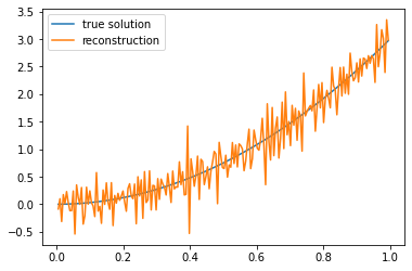
2. Take \(f(x) = x^3 + \epsilon\) with \(\epsilon\) is normally distributed with mean zero and variance \(\delta^2\). Investigate the accuracy of the reconstruction (use np.linalg.solve to solve \(Ku = f\)). Note that the exact solution is given by \(u(x) = 3x^2\). Do you see the regularizing effect of \(n\)?

The code to generate the matrix and its use are given below.

import numpy as np
import matplotlib.pyplot as plt

def getK(n):
    h = 1/(n+1)
    x = np.linspace(h,1-h,n)
    K = h*np.tril(np.ones((n,n)))

    return K,x

n = 200
delta = 1e-3

K,x = getK(n)
u = 3*x**2
f = x**3 + delta*np.random.randn(n)
ur = np.linalg.solve(K,f)

print('|u - ur| = ', np.linalg.norm(u - ur))

plt.plot(x,u,label='true solution')
plt.plot(x,ur,label='reconstruction')
plt.legend()
plt.show()

|u - ur| =  4.068911237154736

3.6.2. Convolution on a finite interval

We can define convolution with a Gaussian kernel on a finite interval \([0,\pi]\) through the initial boundary-value problem

\[ v_t = v_{xx}, \quad v(t,0) = v(t,\pi) = 0,\quad v(0,x) = u(x) \]

with \(f(x) = v(1,x)\). The solution of the initial boundary-value problem is given by

\[ v(t,x) = \sum_{k=1}^{\infty} a_k\exp(- k^2 t)\sin(k x), \]

with \(a_k\) are the Fourier sine coefficients of \(u\):

\[ a_k = \langle u, \sin(k\cdot) \rangle = \frac{2}{\pi}\int_0^{\pi} u(x) \sin (k x) \mathrm{d}x. \]

Assume that we use \( \langle u, v \rangle = \frac{2}{\pi}\int_0^{\pi} u(x) v(x) \mathrm{d}x\) as inner product and define the forward operator \(f = Ku\) in terms of the solution of the IBVP as \(f(x) = v(1,x)\).

---

1. Give the singular system of \(K\), i.e., find \((\sigma_k, u_k, v_k)\) such that \(Ku(x)\) can be expressed as

\[ Ku(x) = \sum_{k=0}^\infty \sigma_k \langle u, v_k \rangle u_k(x). \]

---

We can now define a regularized pseudo-inverse through the variational problem

\[ \min_{u} \|Ku - f\|^2 + \alpha R(u), \]

where we investigate two types of regularization

1. \(R(u) = \|u\|^2,\)

2. \(R(u) = \|u'\|^2.\)

---

2. Show that these lead to the following regularized pseudo-inverses

1. \(K_{\alpha}^\dagger f = \sum_{k=0}^\infty \frac{1}{\sigma_k + \alpha\sigma_k^{-1}}\langle f, u_k \rangle v_k(x).\)

2. \(K_{\alpha}^\dagger f = \sum_{k=0}^\infty \frac{1}{\sigma_k + \alpha k^2\sigma_k^{-1}}\langle f, u_k \rangle v_k(x)\)

hint: you can use the fact that the \(v_k\) form an orthonormal basis for functions on \([0,\pi]\) and hence express the solution in terms of this basis.

---

We can now study the need for regularization, assuming that the Fourier coefficients \(f_k = \langle f, u_k \rangle\) of \(f\) are given.

3. Determine which type of regularization (if any) is needed to satisfy the Picard condition in the following cases (you can set \(\alpha = 1\) for this analysis)

1. \(f_k = \exp(-2 k^2)\)

2. \(f_k = k^{-1}\)

---

4. Compute the bias and variance for \(u(x) = \sin(k x)\) and measurements \(f^{\delta}(x) = Ku(x) + \delta \sin(\ell x)\) for fixed \(k < \ell\) and \(\delta\). Plot the bias and variance for well-chosen \(k,\ell\) and \(\delta\) and discuss the difference between the two types of regularization.

previous

2. Discrete Inverse Problems and Regularization

next

4. A statistical perspective on inverse problems