Magnetic Resonance Imaging
Contents
10. Magnetic Resonance Imaging
10.1. A very brief history of MRI
1946: Felix Bloch and Edward Purcell independently discover the magnetic resonance phenomenon (Nobel Prize in 1952)
1971: Raymond Damadian observes different nuclear magnetic relaxation times between healthy tissue and tumor. Clinical application are envisioned
1973/1974: Paul C. Lauterbur and Peter Mansfield apply gradient magnetic fields to obtain spatial encoding: first MR images (Nobel Prize in 2003)
1980’s: MRI scanners enter the clinics.
1990’s: enlarging field of clinical application, higher magnetic field magnets
2000-present: accelerating acquisition protocols.
At the present, more than 100 million MRI scans are worldwide performed each year. Most common applications include tumors, multiple sclerosis, epilepsy, ischemic stroke, stenosis or aneurysms (MR Angiography), sardiac, musculoskeletal system, brain functioning (functional MRI), MR guided surgery (e.g. MRI-Linac).
10.2. Physical Principles
Central quantity is the magnetization \(\mathbf{m} = (m_x ,m_y ,m_z)^T\in\mathbb{R}^3\), which describes the net effect of nuclei magnetic moments (in the body mostly \(^1\)H) over a small volume at position \(\mathbf{r} = (x, y, z)^T\).
Suppose an external magnetic field \(\mathbf{b}=(b_x,b_y,b_z)^T\) is present, the behavior of the magnetization is given by the following equation (by Felix Bloch):
The quantities \(T_1\), \(T_2\) and \(\rho\) are tissue properties (parameters) and vary depending on the tissue type and structure. This makes it possible to spot abnormalities in tissues. \(\gamma\) is a physical constant (gyromagnetic ratio). The Bloch equation can be written in a more compact form:
This equation can look rather complex at a first glance. To better understand the dynamics involved let’s separate the tissue-parameter (i.e. \(T_1,T_2,\rho\)) dependent and independent parts.
Note that this differential equation is characterized by a skew-symmetric matrix. This is equivalent to a rotation of \(\mathbf{m}\) around the magnetic field vector \(\mathbf{b}\). The remaining part is given by
This differential equation clearly describes two independent exponential decays, one for \(m_{xy}\equiv m_x+\mathrm{i}m_y\) with decay rate \(-1/T_2\) and one for \(m_z\) with rate \(-1/T_1\).
In conclusion: applied, time-dependent magnetic field \(\mathbf{b}\) contributes to rotate the magnetization vector. The tissue properties contribute to different decay (or relaxation) behavior for different tissue types. During an MRI scan, the interplay of these two kind of dynamics makes it possible to generate an image.
10.3. An MRI scan
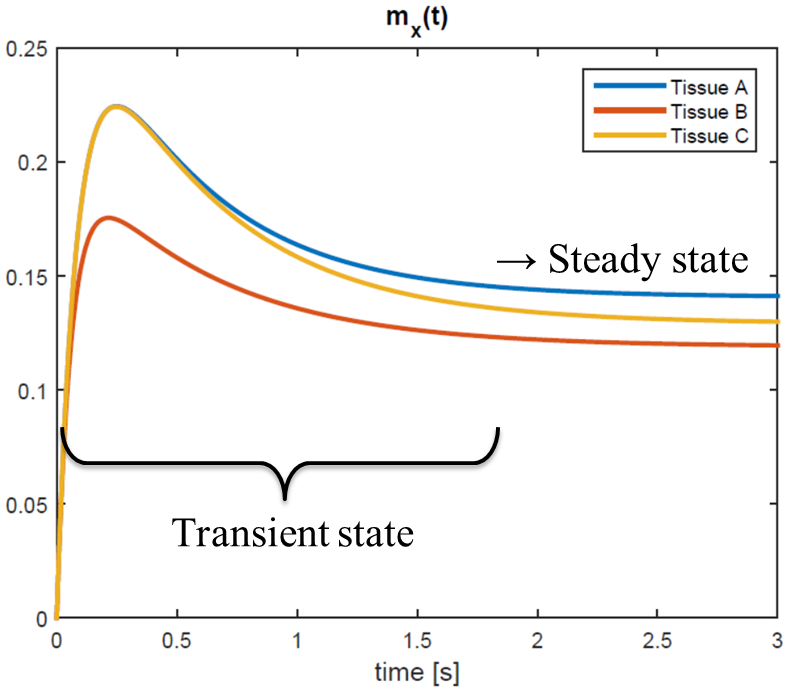
Let’s start by investigating what happens to a single tissue component during an MRI scan. When we lay inside an MRI scanner, the large doughnut-shaped magnet generates a very strong magnetic field in the feet-head direction. By definition, this is the longitudinal, \(z\) component. The transverse component \(m_{xy}\) is randomly distributed over a small volume \(V\) (zero net sum over \(V\)). Only the longitudinal component \(m_z\) is slightly different than 0, but since we can only measure the \(m_{xy}\) component, no signal can be collected.
To measure the magnetic moments, we need them to attain a net transverse magnetization component which differs from 0. Since the \(\mathbf{m}\) is initially aligned along \(z\) we will need a magnetic field component perpendicular to that (remember: the magnetic field \(\mathbf{b}\) contributes to rotate \(\mathbf{m}\) around itself). For simplicity, suppose we superimpose a time-independent magnetic field \(\mathbf{b}\) that is aligned along the \(y\) direction: \(\mathbf{b}(t) = (0,b_y,0)^T\) for each \(t>0\). The Bloch equation (10.2) admits the following solution:
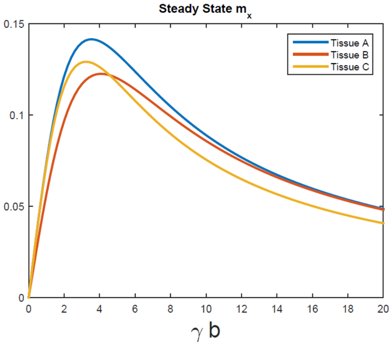
A graph of the solution \(m_{xy}\) for three different combinations of tissue parameters \((T_1,T_2)\) is plotted in Fig. 10.1. What would have happened if we had chosen a different value for the magnetic field \(b_y\)? Let’s have a look at the steady-states solution of the Bloch equation for time-constant magnetic fields. To derive the steady state signal, set \(\text{d}\mathbf{m}/\text{d}t = \mathbf{0}\):
Which leads to
A plot of \(m_{xy}(t)\) for different values of the magnetic field component \(b_y\) is shown in Fig. 10.2. Note that not only the absolute amplitude of each signal changes, but, more importantly, also the relative amplitude (contrast) changes; for instance, for \(\gamma b_y=3\), tissue C gives higher signal than tissue B. At \(\gamma b_y=8\) the situation is inverted. Furthermore, for high magnetic field values, tissue A and B generate the same signal amplitude, which means they cannot be differentiated at all.
To better illustrate this point, I simulated the transverse magnetization for a 2D object made of these three tissue types. See Fig. 10.3.
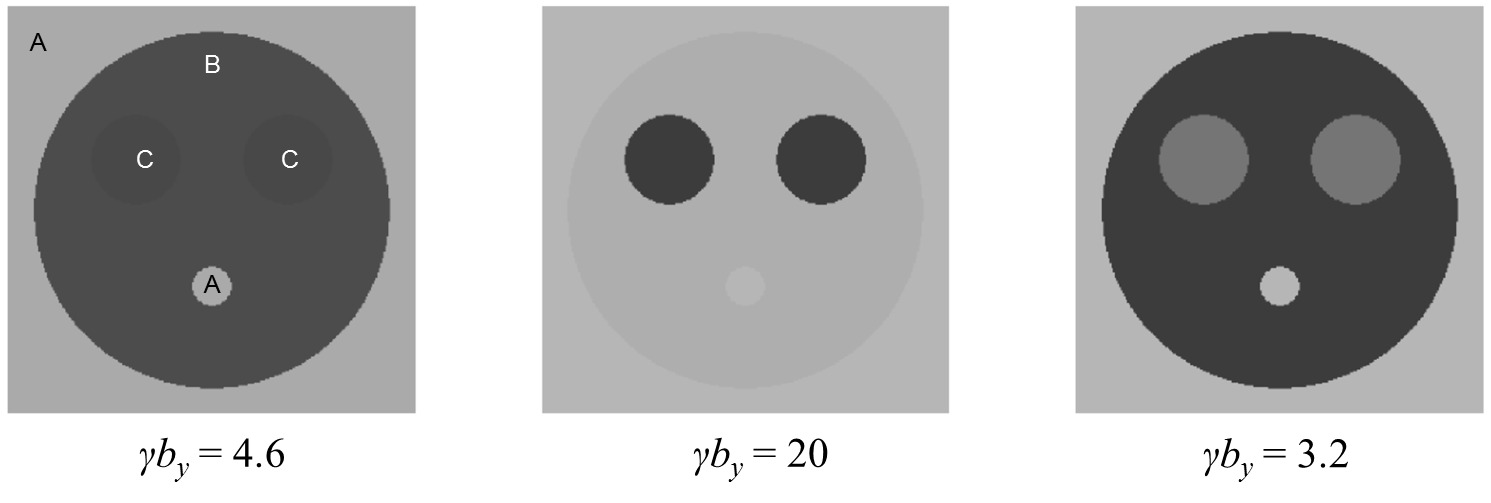
Fig. 10.3 Contrast obtained for di erent experimental settings in a 2D object.
Tuning the scanner parameter \(b_y\) to different levels results in different contrast images. A more realistic, in-vivo illustration of how the scanner settings influence the acquired image is reported in figure Fig. 10.4. Note that the these four images are acquired from the same slice of the same brain! The ability to capture different anatomical and functional characteristics just by changing magnetic field settings makes MRI probably the richest medical imaging modality.
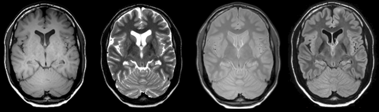
Fig. 10.4 Four different in-vivo contrast images acquired for the same slice of the same brain.
10.4. Imaging
In the previous paragraph we have investigate the behavior of an
individual tissue type. In this section we will see how data from a
whole object (human body) is acquired and processed into an image.
Look again at Fig. 10.1. Once the steady-state condition is reached (in
that specific case for \(t>3\)) the value of \(m_{xy}\) does no longer
change. This allows to encode the spatial information relative to all
position in the image \(m_{xy}(\mathbf{r})\). Spatial encoding can take
some time thus it is important that the state of \(m_{xy}\) is kept
constant during the data acquisition period. We now make a distinction
between two kinds of superimposed magnetic fields:
the Radiofrequency fields are the transverse components \(b_x\) and \(b_y\)
the Gradient fields describe the longitudinal component \(b_z\) and have the form of a gradient: \(b_z(t,\mathbf{r}) = \mathbf{g}(t)\cdot\mathbf{r}\) where \(\mathbf{g}=(g_x,g_y,g_z)\in\mathbb{R}^3\) can be tuned at the user’s discretion. Note that the gradient fields are spatially dependent (this is essential to localize the signal contribution form different positions in the body).
During an MRI scan, these two types of fields are not played out continuously but keep alternating (see Fig. 10.5).
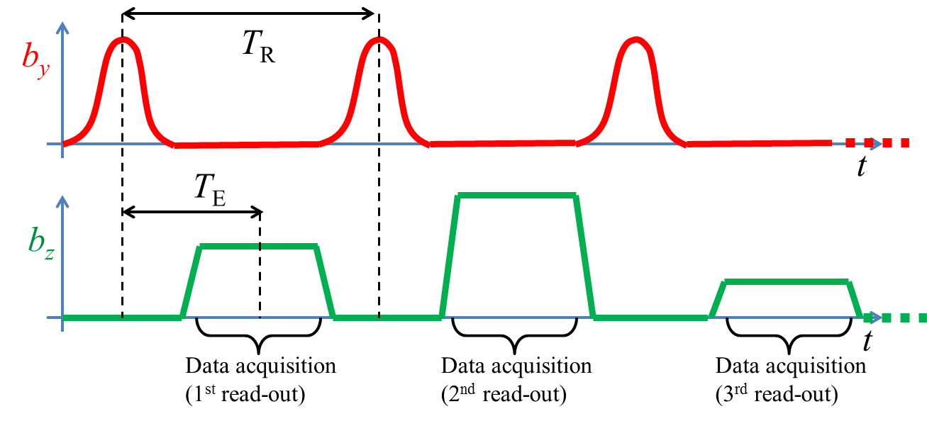
Fig. 10.5 A simple MRI acquisition sequence.
This is a slightly different situation than the scenarios we have previously seen but the physical insights are pretty much the same. The RF fields are used to drive the magnetization to some kind of desired state (for instance a steady-sate) as we have seen in the previous section (remember that, in order to record a signal: \(m_{xy}\neq 0\)). The gradient fields are used to encode the information, i.e. to collect a signal which can be reconstructed into an image. The period of this alternation is called repetition time (\(T_R\)) and the time-distance between the radiofrequency and the gradient blocks is the echo time (\(T_E\)); \(T_R\) and \(T_E\) can be arbitrarily set to modify the contrast type.
Since each data acquisition block (read-out) lasts a very short time (few milliseconds) we can ignore the relaxation effects and study their behavior at the hand of equation (10.3). In particular, suppose that at the start of the acquisition (\(t =t_0\)) we are in a steady-state \(m_{xy}=u\); under effect of the gradient fields, the transverse magnetization will have the following form:
which is of course still a localized signal expression. We will now make the final step toward MR Imaging. In an MRI scanner, radiofrequency receive coils are used to capture the total amount of transverse magnetization present in the object. By using Faraday’s induction law, it can be shown that the signal \(s(t)\) recorded by the coil is proportional to the volumetric integral of all local \(m_{xy}\) contributions:
where we made use of equation (10.5) for the second equality. It is important to realize that the measured signal \(s(t)\) does not directly tell us how the spatial distribution of \(u\) (i.e. the image) look like. In order to reconstruct \(u(\mathbf{r})\) we need to solve the integral equation (10.6). This step is going to be much easier if we rewrite this equation by introducing the following variable:
Note that, for ease of notation, we have dropped the proportionality sign from (10.6) (you could think of it as a global, space-independent factor which scales \(u\)). Obviously, the equation above unveils a Fourier transform relationship between the signal and the image \(u\). To reconstruct the image we can apply inverse (Discrete) Fourier transform to the data \(s\) (see figure Fig. 10.6).
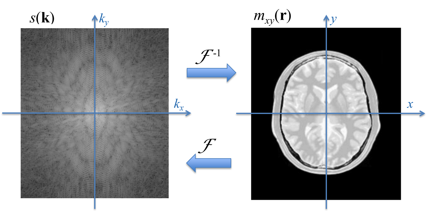
Fig. 10.6 \(k\)-space and image space. The data acquisition process is mathematically equivalent to a Fourier transform F of the image. To reconstruct the image, inverse Fourier transform \(\mathcal{F}^{-1}\) can be applied.
The new variable \(\mathbf{k}\) denotes a spatial frequency term and the
signal can be interpreted as the multi-dimensional frequency
representation of the image. The signal domain is also called the
\(k\)-space.
Equation (10.8) has profound implications not only in the
reconstruction but also in the data acquisition process. Fourier
theory tells which sample point in \(k\)-space need to be acquired in
order to obtain a faithful reconstruction of the true magnetization map
of the body. In particular, the Nyquist criterion states that for an
image of size \(L\times L\) and a desired resolution \(\Delta_s\) in both
directions, samples in \(k\)-space should be acquired at distance \(1/L\)
over the interval \([-1/\Delta_s, + 1/\Delta_s]\). See Fig. 10.7.
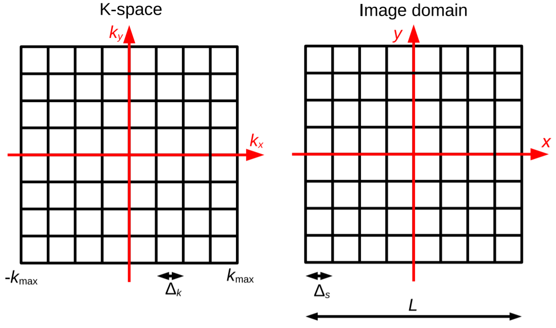
Fig. 10.7 Sampling in \(k\)-space
In conclusion, the MRI acquisition process is characterized by two main components:
Radiofrequency excitations to drive and keep the magnetization into a tissue-dependent state \(u(\mathbf{r})\)
gradient field encoding to collect the signal \(s(\mathbf{k})\) as spatial frequency coefficients of \(u(\mathbf{r})\)
The first component is responsible for the different type of contrast characteristics of the image. The second component make sure that the acquired data can correctly be reconstructed at the desired resolution.
10.4.1. Traversing the \(k\)-space
Let’s have a closer look at the data acquisition component (encoding). This is achieved by ensuring sufficient portion of the \(k\)-space is sampled, with the proper density (Nyquist criterion). In practice, there are several ways to sample the \(k\)-space. Equation (10.7) shows the direct relationship between the somehow abstract concept of \(k\)-space coordinate and the practical, actually produced gradient field \(\mathbf{g}(t)\); given a desired sampling trajectory, \(\mathbf{k}(t)\), we can easily derive the corresponding scanner’s input parameter \(\mathbf{g}(t)\).
As a very simple example, consider a 2D cartesian encoding scheme with equal time-steps \(\Delta_t\) (Fig. 10.8).
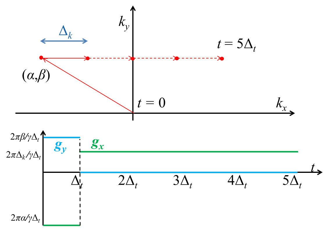
Fig. 10.8 Top: a very simple 2D cartesian trajectory in red. Bottom: corresponding gradient waveforms in green and blue.
To traverse a single line, parallel to the \(k_x\) axis and given \(k_y=\beta\) coordinate, we first impose
Assuming a constant \(g_y\), this leads to \(g_y=\frac{2\pi\beta}{\gamma\Delta_t}\). For \(k_x\) a similar argument shows that, in order to move to the \(k_x = \alpha\) position at \(t=\Delta_t\): \(g_x=\frac{2\pi}{\gamma\Delta_t}\alpha\). Thus, for \(t\in[0,\Delta_t]\), we set \(\mathbf{g}=(\frac{2\pi}{\gamma\Delta_t}\beta,\frac{2\pi}{\gamma\Delta_t}\alpha)^T\). At time \(t = \Delta_t\) we have \(\mathbf{k}(\Delta_t)=(\alpha,\beta)\). We start acquiring data keeping \(k_y\) constant, thus from now on, \(g_y=0\) (why?). Assume that \(\Delta_k\) is the desired distance between consecutive \(k\)-space locations. For \(g_x\) we need to solve:
Thus, for each \(t>\Delta_t\) we set \(\mathbf{g}=(\frac{2\pi}{\gamma\Delta_t}\Delta_k,0)^T\). See Fig. 10.8 for a pictorial illustration. Although the cartesian sampling is by far the most commonly used scheme for clinical MRI exams, other trajectories are gradually entering the MRI practice. See Fig. 10.9 for other 2D and 3D examples.
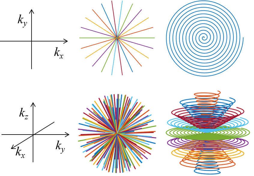
Fig. 10.9 Examples of 2D and 3D non-cartesian \(k\)-space trajectories
10.4.2. Image reconstruction: beyond the Fast Fourier Transform
We discretize the signal equation (10.8) as
where we used the following notation:
\(\mathbf{s}\): the vector of signal samples (\(k\)-space data)
\(\mathbf{u}\): the vector of image values (i.e. a discretized version of \(u(\mathbf{r})\) )
\(\mathcal{F}\): the \(N\)-dimensional sampling (Fourier transform) operator: \(\mathcal{F}_{i,j} = \exp\left(-2\pi\text{i}\mathbf{k}_i\cdot \mathbf{r}_j\right)\nu\) with volume element \(\nu\).
For cartesian, equidistant samples of \(k\)-space, the operator \(\mathcal{F}\) in equation (10.9) is unitary and can be implemented by the Fast Fourier transform (FFT) algorithm. To reconstruct \(\mathbf{u}\), the inverse FFT can be applied: \(\mathbf{u} = \mathcal{F}^{-1}\mathbf{s}\) where in this case \(\mathcal{F}^{-1}=\mathcal{F}^H\). This is :
computationally efficient; applying FFT to a \(N\)-long array scales with \(N\log_2 N\) while naive implementation would scale with \(N^2\).
memory efficient, because no operator needs to be stored.
For other, non-cartesian trajectories, the solving strategies are more complex. First of, all, note that \(\mathcal{F}\) in most cases will not be a unitary, square operator. The problem will be solved by minimizing some norm of the residual, usually the squared \(\ell_2\) norm (least-squares problems):
It is interesting to give a closer look at this numerical problem. Suppose we acquire data according to a 2D spiral trajectory, which can be parametrized as:
with \(\alpha,\beta\in\mathbb{R}\).
Fig. 10.10 shows a portion of the samples at the \(k\)-space center. For design constraints, points in the middle are mutually much closer. As a consequence, many rows in the operator \(\mathcal{F}\) are almost equal, leading to problems with respect to linear dependence and orthogonality. This is more clearly demonstrated in Fig. 10.10 which show the spectrum (singular values) of \(F\); the singular values are not equal (a characteristic of orthogonal operators) but gradually decay to machine precision level after a while, leading to ill-conditioning.
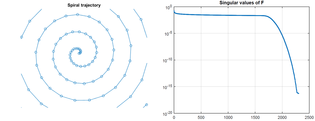
Fig. 10.10 Magnified portion of \(k\)-space samples for a 2D spiral trajectory and the spectrum of the corresponding \(\mathcal{F}\) operator. Note the decaying singular values.
To mitigate this problem, regularization needs to be applied. This is usually done by introducing a penalty \(R\) on the computed solution \(\mathbf{u}\):
The most common choice for \(R\) is \(R(\mathbf{u})=\|\mathbf{u}\|_2^2\) (Tikhonov regularization). Other common choices will be shown below.
10.4.3. Acceleration techniques
Note that the sampling is a time-dependent process; if two consecutive samples are acquired at \(\Delta_t\) distance, acquisition of \(N\) samples along the trajectory will take \(N\Delta_t\) amount of time. In practice, \(\Delta_t\) is in the order of \(10^{-6}\). Acquiring 2D image of size \(256\times 256\) will require \(256^2\approx 65,000\) samples, thus a fraction of a second.
However, a single 2D image is not sufficient for diagnosis and either several stacked 2D images (slices) are needed or a full-3D acquisition. In both cases, the amount of data needed is multiplied by a factor close to 100 (either 100 2D slices or an additional dimension). This time, the acquisition would last several seconds or even minutes, depending on the sequence timings \(T_R\) and \(T_E\). In this analysis, I consider only the duration of the sampling component, remember (cf. Fig. 10.5) that also RF events need to be played out in order to drive and keep the magnetization in a desired state.
Toward the end of the previous century, a solution strategy was found to accelerate the scans. It all began around the year 1990 when multiple receive channels were introduced to increase the signal-to-noise-ratio (SNR). However, MRI scientists soon realized that using multiple coils could also allow for shorter data-acquisition protocols.
Parallel imaging in MRI works in the following way. Due to electromagnetic interference effects (electromagnetism is a wave phenomenon), each \(p\)-th receiver coil is characterized by its own radiofrequency field (sensitivity map) \(c^p(\mathbf{r})\). Therefore, the signal equation has to be slightly modified:
where \(C^p\) is a diagonal matrix with \(C^p_{n,n} = c^p(\mathbf{r}_n)\) and \(\mathbf{s}^p\) is the signal from the individual coil. The image is obviously the same for all receive coils, thus it can be reconstructed by solving the joint reconstruction system:
which we can be solved as
where \(\mathbf{s}\) now denotes the concatenated signal from all coils and \(F\) the joint linear multi-coil model.
Note that the operator \(F\) is a tall operator, that is, there are (many) more data samples (rows) than unknowns (columns). It makes therefore sense to under-sample \(\mathcal{F}\) by deleting rows, that is, skipping points in \(k\)-space. Since the sensitivity matrices \(C^p\) are not equal, the resulting joint operator \(F\) should still have full rank, making the inversion possible. Of course, the practical consequence of under-sampling the \(k\)-space is a much shorter acquisition protocol. Although there are limits to the under-sampling level as set by the number of coils, geometry and trade-off SNR/time, acceleration factors between 2 and 5 are quite common. For this reason, parallel imaging is nowadays applied in almost all clinical protocols.
The most recent advance in accelerated protocols is the introduction of compressed sensing. Basically, the reconstruction problem (10.10) is solved with a non-linear regularization term \(R\), usually in the form \(R(\mathbf{u})=\|\mathbf{u}\|_1\), \(R(\mathbf{u})=\|W\mathbf{u}\|_1\) or \(R(\mathbf{u})=TV(\mathbf{u})\) where \(W\) denotes a sparsity operator and \(TV\) the total variation functional. The sampling strategy needs to be adapted to guarantee incoherence, which can be explained as a noise-like behavior of under-sampling artifacts. Pseudo-randomization of the \(k\)-space trajectory with higher sampling density in the middle is usually the most practical choice. See Fig. 10.11.
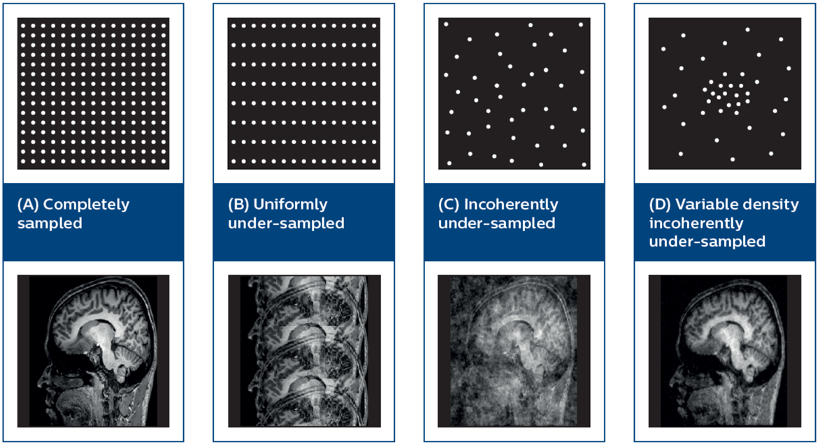
Fig. 10.11 Compressed sensing in MRI. Top: illustrative sketch of 2D k-space sampling strategy. Bottom: Reconstruction by Compressed sensing. Note that the variable-density randomized sampling (right) gives the best reconstruction quality. Image taken from Geerts-Ossevoort et al (Philips). Compressed Sense (2018).
Compressed sensing has recently entered clinical practice and showed to further accelerate exams by about 40%.
10.5. Exercises
10.5.1. Rotation
Can you prove that (10.3) defines a rotation and that the rotation axis is aligned along \(\mathbf{b}\)? What is the rotation angle? HINT: Write the solution to the differential equation in terms of the matrix-exponential and have a look at Rodrigues’ rotation formula.
10.5.2. Decay
Rewrite (10.4) as two independent equations, one for the transverse component \(m_{xy}\) and one for the longitudinal component \(m_z\). Find the solution for both equations for a generic time point \(t\) with initial values \(m_{xy}(0) =m_{xy}^0\) and \(m_z(0) = m_z^0\). What happens in the limit case \(t\rightarrow +\infty\)?
10.6. Assignment
10.6.1. MRI-reconstruction
Set up a regularised inversion for an MRI scan with standard cartesian sampling. As test data you can use skimage.data.brain. You may assume that the data are noisy (subsampled) versions of the Fourier transform of the image slices. Can you get rid of aliasing artefacts using appropriate Tikhonov regularisation?