9. Wavefield Imaging¶

In many applications, acoustic or electromagnetic waves are harnessed to see things; under-water acoustics, radar, sonar, medical ultrasound, ground penetrating radar, seismic imaging, global seismology. In some of these applications the measurements are passive; we record waves that are emitted by the object of investigation and we try to infer its location, size, etc. In active measurements, waves are generated and the response of the object is recorded. An example of such an application is shown in Fig. 9.1.

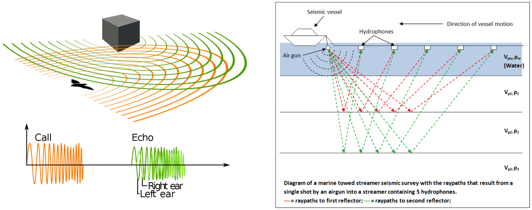
Fig. 9.1 Acquisition setup of a bat and an active marine seismic survey.¶

In order to treat the inverse problem, we must first understand the forward problem. In its most rudimentary form, the wave-equation is given by

(9.1)¶\[L[c]v(t,x) = q(t,x),\]

with

\[ L[c] = \left[\frac{1}{c(x)^2}\frac{\partial^2}{\partial t^2} - \nabla^2 \right], \]

and where $v : \mathbb{R} \times \mathbb{R}^n \rightarrow \mathbb{R}$ denotes the wavefield, $c : \mathbb{R}^n \rightarrow \mathbb{R}$ is the speed of propagation and $q : \mathbb{R} \times \mathbb{R}^n \rightarrow \mathbb{R}$ is a source term. We will assume that the source has compact support in both space and time and is square integrable.

To define a unique solution of (9.1) we need to supply boundary and initial conditions. In the applications discussed above one typically considers an unbounded domain ($x \in \mathbb{R}^n$) and Cauchy initial conditions $v(0,x) = 0$, $\frac{\partial v}{\partial t}(0,x) = 0$.

In scattering experiments it is common to rewrite the wave-equation in terms of an incoming and a scattered wavefield, $v = v_i + v_s$, and a scattering potential, $u(x) = c(x)^{-2} - c_0^{-2}$:

(9.2)¶\[L[c_0]v_i(t,x) = q(t,x), \quad L[c_0]v_s(t,x) = -u(x)\frac{\partial^2 v}{\partial t^2}(t,x).\]

Under a weak scattering assumption, we may ignore the interaction of $u$ and $v_s$ and replace $v$ in (9.2) by $v_i$.

The measurements are typically taken to be the (scattered) wavefield restricted to $[0,T] \times \Delta$ where $\Delta \subset \mathbb{R}^n$ may be a manifold or a set of points. The data may then be denoted by $f(t,r)$. In active experiments, it is common practice to consider measurements for a collection of source terms. The sources may be point-sources, in which case $q(t,x) = w(t)\delta(x - s)$ with $s \in \Sigma$. Alternatively, the incident field $v_i$ may be given and parametrized by $s \in \Sigma$. We may then denote the data by $f(t,s,r)$ with $s\in \Sigma$, $r\in \Delta$ and $t\in [0,T]$.

Based on this basic setup, we will discuss three possible inverse problems:

Inverse source problem: Recover the source $q$ from the measurements for known (and constant) $c(x)\equiv c_0$.
Inverse scattering: Recover the scattering potential $u(x)$ from measurements of the scattered field for multiple (known) sources, assuming that $c_0$ is known.
Waveform tomography: Recover $c(x)$ from measurements of the total wavefield for multiple (known) sources.

Below you will find some typical examples of inverse problems that come up in practice.

Earth-quake localization: An earthquake described by a source term $w(t)q(x)$ is recorded by multiple seimosgraphs at locations $\Delta = \{r_k\}_{k=1}^n$. The goal is to recover $q$ in order to determine the location of the earthquake.
Passive sonar: Soundwaves emitted from an unidentified target are recorded using an array $\Delta = \{x_0 + rp \, | \, r\in[-h,h] \}$, where $p\in\mathbb{S}^2$ denotes the orientation of the array and $h$ its width. The goal is to recover the source term $w(t)q(x)$ to determine the origin and nature of the source.
Radar imaging: Incident plane waves, parametrized by direction $s \in \Sigma \subset \mathbb{S}^{2}$, are send into the medium and their reflected response is recorded by an array. The goal is retreive the scattering potential.
Full waveform inversion: In exploration seismology, the goal is to recover $c$ from measurements of the total wavefield on the surface: $\Sigma = \Delta = \{x \,|\, n\cdot x = 0\}$.
Ultrasound tomography: The goal is to recover $c$ from the total wavefield for sources and receivers surrounding the object.

A few prominent examples of acquisition setups we will consider here are the following:

Point-sources: $q(t,x) = w(t)\delta(x - s)$. \item Incoming plane waves with frequency $\omega$ and direction $\xi$: $v_i(t,x) = \sin(\omega(t - \xi\cdot x/c))$
Point-measurements along a hyperplane: $\Delta = \{x \in \mathbb{R}^n\, |\, n\cdot x = x_0\}$.
Point-measurements on the sphere: $\Delta = \{x \in \mathbb{R}^n \, | \, \|x\| = \rho\}$.

We will further assume that the quantities of interest are compactly supported in both space and time and that the measurement time $T$ is large enough to capture all the required information. This situation is sketched in Fig. 9.2.

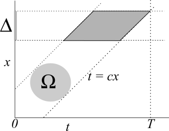
Fig. 9.2 All information on the compactly supported source term is captured in the light cone defined by $t = c\cdot x$. We assume that $T$ is large enough to capture the complete intersection of the light cone with $\Delta$.¶

9.1. Forward modelling¶

9.1.1. Analytic solution¶

For a general source term we may express the solution as a convolution

\[ v(t,x) = \int\!\!\int g(t-t',x,x') q(t',x')\mathrm{d}t'\mathrm{d}x', \]

where $g$ is the Green function, obeying

\[ L[c]g(t,t',x,x') = \delta(t-t')\delta(x-x'). \]

For $c(x) \equiv c$ we have $g(t,t',x,x')\equiv g(t-t',x-x')$ and the Green functions are given by:

\[ g(t,x) = \frac{1}{2c}H(t - |x|/c), \]

for $n=1$,

\[ g(t,x) = \frac{1}{2\pi c\sqrt{c^2t^2 - |x|^2}}H(t - |x|/c), \]

for $n=2$, and

\[ g(t,x) = \frac{1}{4\pi |x|} \delta(t - |x|/c), \]

for $n=3$. Note that these are the causal Green functions; they propagate information forward in time. The *a-causal* or time-reversed Green functions also satisfy the wave-equation.

The solution for non-constant $c$ can be constructed by solving an integral equation

\[ v = g_0*q - g_0*\left(u\cdot \frac{\partial^2 v}{\partial t^2}\right), \]

where $*$ denotes convolution, $g$ is the Green function for $c(x) \equiv c_0$ and $u = c^{-2} - c_0^{-2}$.

9.1.2. Numerical modelling¶

For non-constant $c$, such closed-form expression are generally not available. The most basic method for solving the wave equation numerically is the Leap-Frog method. For $n=1$, the method may be expressed as follows. Introducing $v_{ij} \equiv v(i\Delta t, j\Delta x)$ we have

\[ \frac{v_{i+1,j} - 2v_{i,j} + v_{i-1,j}}{c_{ij}^2\Delta t^2} - \frac{v_{i,j+1} - 2v_{i,j} + v_{i,j-1}}{\Delta x^2} = q_{ij} + \mathcal{O}(\Delta x^2) + \mathcal{O}(\Delta t^2). \]

We need to truncate the spatial domain to $[-L,L]$ in order to compute solutions. We need boundary conditions that will let waves leave the domain with reflecting of the artificial boundary. The simplest are so-called radiation boundary conditions, that impose a one-way wave equation in the direction normal to the boundary:

\[ \frac{\partial v}{\partial t}(t,\pm L) = \pm c(\pm L)\frac{\partial v}{\partial x}(t,\pm L), \]

which can be discretized using finite-differences as well.

Ignoring the higher order terms leads to

\[ \widetilde v_{i+1,j} = 2\widetilde v_{i,j} - \widetilde v_{i-1,j} + \frac{c_{ij}^2\Delta t^2}{\Delta x^2}\left(\widetilde v_{i,j+1} - 2\widetilde v_{i,j} + \widetilde v_{i,j-1} + \widetilde q_{i,j}\right),\quad j=-J+1, \ldots, J-1, \]

and

\[ \widetilde{v}_{i+1,-J} = \widetilde{v}_{i,-J} + \frac{c_{i,-J}\Delta t}{\Delta x}\left(\widetilde v_{i,-J+1} - \widetilde v_{i,-J}\right), \]

\[ \widetilde{v}_{i+1,J} = \widetilde{v}_{i,J} + \frac{c_{i,J}\Delta t}{\Delta x}\left(\widetilde v_{i,J} - \widetilde v_{i,J-1}\right), \]

with $\widetilde v_{0,j} = \widetilde v_{1,j} = 0$ and $\widetilde q_{i,j} = \Delta x^2 q(i\Delta t, j \Delta x)$.

The accuracy of the approximation follows directly from the higher order terms we left out. Another important aspect is stability, which tells us how errors propagate. Since the equations are all linear, errors will propagate according to the same recursion relation. One way of studying this is von Neumann stability analysis, where we study the behaviour of individual components of the error: $e_{ij} = g^i\exp(\imath j\theta)$. This yields to following quadratic equation for $g$:

\[ g^2 - 2g + 1 = 2\gamma g(\cos(\theta\Delta x)-1), \]

with $\gamma = \frac{c\Delta t}{\Delta x}$. To ensure stability, we need $|g|\leq 1$ for all $\theta$, which requires that $\gamma\leq 1$.

9.2. Analysis¶

9.2.1. Source localization¶

Define forward map

\[ f = Kq, \]

with

\[ Kq(t,x) = \int\int g(t-t',x-x')q(t',x')\mathrm{d}x'\mathrm{d}t'. \]

Data are measured at locations $x \in \Delta$ and $t\in[0,T]$.

Uniqueness. Can we find sources $r_0$ for which $\|Kr_0\| = 0$? Yes! First define $w_0(t,x)$ compactly supported in $[0,T] \times \Omega$ so that $w_0(t,x) = 0$ for $x\in P$ and set

\[ r_0(t,x) = L[c]w_0(t,x), \]

then $Kr_0 = w_0$, which is zero for $x\in \Delta$ and $t\in[0,T]$.

Stability. We can also construct sources that radiate an arbitraliy small amount of energy by picking $w_{\epsilon}$ such that $\|w_{\epsilon}\| = \mathcal{O}(\epsilon)$ and $\|Lw_{\epsilon}\| = \mathcal{O}(1)$ as $\epsilon\downarrow 0$. Then $K(q + r_{\epsilon}) = d + w_{\epsilon}$ and small perturbation in data leads to large perturbation in the solution.

This will be explored in more detail in the assignments.

9.2.2. Inverse scattering¶

Under the weak scatterin assumption, the scattered field is given by

\[ v_s(t,x) = \int\int u(x')\frac{\partial^2 v_i}{\partial t^2}(t',x')g(t-t',x,x')\mathrm{d}t'\mathrm{d}x', \]

which we measure at $x \in \Delta$ and $t\in [0,T]$. Can we construct $u$ such that $u(x')\frac{\partial^2 v_i}{\partial t^2}(t',x')$ is a non-radiating source? Following the approach described earlier, we start with $w_0(t,x)$ which is zero for $x \in \Delta$. Then, we want to decompose the resulting non-radiating source in two components: $u \cdot \frac{\partial^2 v_i}{\partial t^2}$. We can probably manage this for one incoming wavefield, but can we find a potential that is non-scattering for multiple incoming waves? In the assignments we will explore non-radiating sources in more detail.

9.3. Reconstruction¶

9.3.1. Inverse source problem¶

We study a variant of the inverse source problem in which $q(t,x) = \delta(t)u(x)$ and $u$ is compactly supported on $\Omega \subset \mathbb{R}^n$. The foward operator for constant $c$ is given by

\[ Ku(t,x) = \int_{\Omega} u(x')g(t,x-x') \mathrm{d}x', \]

with measurements on the sphere with radius $\rho$. A popular techique to solve the inverse problem is backpropagation, which is based on applying the adjoint of the forward operator to the data. The adjoint operator in this case is given by

\[ K^* f(x) = \int_{\Delta}\int_0^T g(t',x'-x)f(t',x') \mathrm{d}x'\mathrm{d}t'. \]

We see that $p = K^* f$ can be obtained by solving

\[ L[c]w(t,x) = \int_{\Delta}f(t,x')\delta(x-x')\mathrm{d}x', \]

using the time-reversed Green function and evaluating at $t=0$, i.e. $p(x) = w(0,x)$.

To see why this works, we study the normal operator $K^*K$. In the temporal Fourier domain, for $c = 1$, the operator becomes

\[ \widehat{f}(\omega,x) = \int_{\Omega} u(x') \frac{\exp(\imath\omega|x-x'|)}{|x-x'|}\mathrm{d}x', \]

and

\[ u(x) = \int \int_{\Delta} \widehat{f}(\omega,x') \frac{\exp(-\imath\omega|x'-x|)}{|x'-x|} \mathrm{d}x'\mathrm{d}\omega. \]

so

\[ K^* Ku(x) = \int \int_{\Delta}\int_{\Omega} f(x') \frac{\exp(\imath\omega|x''-x'|)}{|x''-x'|} \frac{\exp(-\imath\omega|x''-x|)}{|x''-x|} \mathrm{d}x'\mathrm{d}x''\mathrm{d}\omega. \]

For $|x''| \gg |x|$ we can approximate it as $|x'' - x| \approx |x''| + x\cdot x''/|x''|$ and likewise for $|x'' - x'|$. This is called the far-field approximation. Introducing $\xi'' = x''/|x''| = x''/\rho$ on the unit sphere, we find

\[ K^* {K}u(x) = \rho\int_{\Omega} u(x') \int\int\exp(\imath\omega \xi''\cdot(x'-x)) \mathrm{d}\xi''\mathrm{d}\omega\mathrm{d}x'. \]

The kernel

\[ k(x-x') = \int\int \exp(\imath\omega \xi''\cdot(x'-x)) \mathrm{d}\xi''\mathrm{d}\omega, \]

is sometimes refered to as the point-spread function.

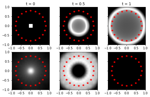
Under ideal conditions, i.e, measurements are available for all frequencies $\omega\in\mathbb{R}$, integration over $\omega$ yields

\[ k(x) = \int \delta(\xi\cdot x) \mathrm{d}\xi. \]

We only get contributions to the integral for directions orthogonal to $x$, because $\delta(\xi\cdot x)=0$ whenever $\xi\cdot x \not=0$. We thus integrate over a circle only. Substituting $\xi \cdot x = |\xi| |x| \cos \theta = |x|\cos \theta$ we obtain

\[ k(x) = \frac{1}{|x|}\int_0^{2\pi} \delta(|x|\cos\theta) \mathrm{d}\theta = \frac{1}{|x|}. \]

Thus with a perfect acquisition we have $k(x' - x) = \frac{1}{|x - x'|}$. Since this corresponds to the Green function of the Poisson equation, it suggests that we may retrieve $u$ by applying a filter to the backprojected data:

\[ u = \nabla^2 (K^*f). \]

This filtering can also be implemented in the Fourier domain by multiplying by $|\xi|^2$. An example is shown below.

import numpy as np
import matplotlib.pyplot as plt
import scipy.sparse as sp
from scipy.ndimage import laplace

def solve(q,c,dt,dx,T=1.0,L=1.0,n=1):
    '''Solve n-dim wave equation using Leap-Frog scheme: u_{n+1} = Au_n + Bu_{n-1} + Cq_n'''
    # define some quantities
    gamma = dt*c/dx
    nt = int(T/dt + 1)
    nx = int(2*L/dx + 2)
    #
    q = np.resize(q,(nx**n,nt))
    # define matrices
    A,B,C,L = getMatrices(gamma,nx,n)

    # main loop
    u = np.zeros((nx**n,nt))

    for k in range(1,nt-1):
        u[:,k+1] = A@u[:,k] + L@u[:,k] + B@u[:,k-1] + (dx**2)*C@q[:,k]

    return u

def getMatrices(gamma,nx,n):

    # setup matrices
    l = (gamma**2)*np.ones((3,nx))
    l[1,:] = -2*(gamma**2)
    l[1,0] = -gamma
    l[2,0] = gamma
    l[0,nx-2] = gamma
    l[1,nx-1] = -gamma

    if n == 1:
        a = 2*np.ones(nx)
        a[0] = 1
        a[nx-1] = 1

        b = -np.ones(nx)
        b[0] = 0
        b[nx-1] = 0

        c = (gamma)**2*np.ones(nx)
        c[0] = 0
        c[nx-1] = 0

        L = sp.diags(l,[-1, 0, 1],shape=(nx,nx))

    else:
        a = 2*np.ones((nx,nx))
        a[0,:] = 1
        a[nx-1,:] = 1
        a[:,0] = 1
        a[:,nx-1] = 1
        a.resize(nx**2)

        b = -np.ones((nx,nx))
        b[0,:] = 0
        b[nx-1,:] = 0
        b[:,0] = 0
        b[:,nx-1] = 0
        b.resize(nx**2)

        c = (gamma)**2*np.ones((nx,nx))
        c[0,:] = 0
        c[nx-1,:] = 0
        c[:,0] = 0
        c[:,nx-1] = 0
        c.resize(nx**2)

        L = sp.kron(sp.diags(l,[-1, 0, 1],shape=(nx,nx)),sp.eye(nx)) + sp.kron(sp.eye(nx),sp.diags(l,[-1, 0, 1],shape=(nx,nx)))

    A = sp.diags(a)
    B = sp.diags(b)
    C = sp.diags(c)

    return A,B,C,L

# parameters
L = 1.0
T = 1.0
dx = 1e-2
dt = .5e-2
nt = int(T/dt + 1)
nx = int(2*L/dx + 2)
c = 1

# define source term
u = np.zeros((nx,nx))
u[nx//2 - 10:nx//2+10,nx//2 - 10:nx//2+10] = 1
q = np.zeros((nx*nx,nt))
q[:,1] = u.flatten()

# forward solve
w_forward = solve(q,c,dt,dx,T=T,L=L,n=2)

# sample wavefield
theta = np.linspace(0,2*np.pi,20,endpoint=False)
xs = 0.8*np.cos(theta)
ys = 0.8*np.sin(theta)
I = np.ravel_multi_index(np.array([[xs/dx + nx//2],[ys//dx + nx//2]],dtype=np.int), (nx,nx))
d = w_forward[I,:]

# define adjoint source
r = np.zeros((nx*nx,nt))
r[I,:] = d
r = np.flip(r,axis=1)

# adjoint solve
w_adjoint = solve(r,c,dt,dx,T=T,L=L,n=2)

# plot
fig, ax = plt.subplots(nrows=2, ncols=3, figsize=(8, 5), sharey=True)
plt.gray()

ax[0,0].plot(xs,ys,'r*')
ax[0,0].imshow(w_forward[:,2].reshape((nx,nx)), extent=(-L,L,-L,L))
ax[0,0].set_title('t = 0')
ax[0,1].plot(xs,ys,'r*')
ax[0,1].imshow(w_forward[:,101].reshape((nx,nx)), extent=(-L,L,-L,L))
ax[0,1].set_title('t = 0.5')
ax[0,2].plot(xs,ys,'r*')
ax[0,2].imshow(w_forward[:,200].reshape((nx,nx)), extent=(-L,L,-L,L))
ax[0,2].set_title('t = 1')

ax[1,0].plot(xs,ys,'r*')
ax[1,0].imshow(w_adjoint[:,200].reshape((nx,nx)), extent=(-L,L,-L,L))
ax[1,1].plot(xs,ys,'r*')
ax[1,1].imshow(w_adjoint[:,101].reshape((nx,nx)), extent=(-L,L,-L,L))
ax[1,2].plot(xs,ys,'r*')
ax[1,2].imshow(w_adjoint[:,2].reshape((nx,nx)), extent=(-L,L,-L,L))

plt.show()

/var/folders/g2/z5xkdjy513j76nkltmmxlkp00000gn/T/ipykernel_24865/1891252179.py:23: DeprecationWarning: `np.int` is a deprecated alias for the builtin `int`. To silence this warning, use `int` by itself. Doing this will not modify any behavior and is safe. When replacing `np.int`, you may wish to use e.g. `np.int64` or `np.int32` to specify the precision. If you wish to review your current use, check the release note link for additional information.
Deprecated in NumPy 1.20; for more details and guidance: https://numpy.org/devdocs/release/1.20.0-notes.html#deprecations
  I = np.ravel_multi_index(np.array([[xs/dx + nx//2],[ys//dx + nx//2]],dtype=np.int), (nx,nx))

9.3.2. Inverse scattering¶

Assuming point sources for the incident field, $c = 1$, and a compactly supported $u$, we can express the forward operator as

\[ Ku(t,r,s) = \int_{\Omega} u(x) \frac{\delta''(t - |x - r| - |x - s|))}{|x - r||x - s|}\mathrm{d}x, \]

so the data $f(t,s,r)$ is the integral of the scattering potential, $u$, along an ellips. Conversely, we can think of the response of a single scattering point $x'$ as a hyperbola in $(t,s,r)$. This is illustrated in Fig. 9.3.

The adjoint operator here is given by

\[ K^* f(x) = \int_\Delta \int_\Sigma \int_{0}^T f(t,r,s)\frac{\delta''(t - |x - r| - |x - s|))}{|x - r||x - s|} \mathrm{d}t\mathrm{d}s\mathrm{d}r. \]

As with the inverse source problem, applying the adjoint already yields an image. This is called migration in practice.

The foward operator has a nice expression in the Fourier domain when using far field measurements. The derivation is left as an excersise.

Fig. 9.3 A single data point $f(t,s,r)$ is the integral of the scattering potential along an ellips: $|x - s| + |x - r| = t$. Likewise, a single point of $f(x)$ contributes to $d$ along a hyperola $t = |x - s| + |x - r|$.¶

9.3.3. Waveform tomography¶

Here, we aim to recover $c$ directly from a non-linear equation

\[ K(c) = f, \]

where $K$ solves $L[c]v = \delta(\cdot - s)w$ and samples the solution. i.e.,

\[ f(t,s,r) = \int g(t-t',r,s)w(t')\mathrm{d}t' \]

for $t\in [0,T]$, $s\in \Sigma$ and $r\in\Delta$.

We can solve such a non-linear equation using Newton’s method:

\[ c_{k+1} = c_k - D{K}(c_k)^{-1}({K}(c_k) - d), \]

where $DK(c_k)$ denotes the Fréchet derivative which generalizes the notion of a derivative and obeys

\[ \lim_{\|h\|\rightarrow 0} \frac{\|K(c + h) - {K}(c) - DK(c)h\|}{\|h\|} = 0. \]

We find

\[ DK(c)\delta c = -\int\int \frac{\delta c (x')}{2c(x')}\frac{\partial^2 v}{\partial t^2}(t',x')g(t-t',x-x')\mathrm{d}t'\mathrm{d}x', \]

where the incident field, $v$, satisfies $L[c]v = \delta(\cdot - s)w$. In a finite-dimensional setting, $DK$ would be the Jacobian of $K$.

Approximating the inverse using backprojection we obtain

\[ c_{k+1} = c_k - \alpha_k DK(c_k)^{\dagger}(K(c_k) - d), \]

where $\alpha_k$ is a scaling factor. Again, we see that backprojection plays a prominant role. It turns out that this iteration is equivalent to a steepest descent method applied to $J(c) = \|K(c) - d\|^2$.

9.4. Exercises¶

9.4.1. Inverse source problem¶

Take $n=1$, $c=1$ and source term $\delta(t)u(x)$ with $u$ square integrable and supported on $[-\frac{1}{2},\frac{1}{2}]$ and measurements at $x = 1$ for $t\in [0,T]$.

Show that the forward operator can be expressed as

\[ f(t) = Ku(t) = \int_{1-t}^{\frac{1}{2}} u(x')\mathrm{d}x', \]

and that the operator is bounded.

Answer

For $n = 1$ the solution to the wave equation with the given source term is given by

\[v(t,x) = \frac{1}{2}\int_{-1/2}^{1/2} \int \delta(t')u(x') H(t - t' - |x - x'|)\mathrm{d}t'\mathrm{d}x' = \frac{1}{2}\int u(x) H(t - |x - x'|) \mathrm{d}x'.\]

For measurements at $x = 1$ this simplifies to

\[f(t) = v(t,1) = \frac{1}{2}\int_{-1/2}^{1/2} u(x') H(t - |1 - x'|) \mathrm{d}x'.\]

This leads to the desired expression becuase we need $t \geq (1-x')$. To show that this a bounded operator consider

\[\|f\|^2 = \int_0^T \left(\frac{1}{2}\int_{\max(\min(1-t,1/2),0)}^{1/2} u(x')\mathrm{d}x'\right)^2 \mathrm{d}t \leq \frac{1}{4}\int_0^T (1/2-\max(\min(1-t,1/2),0))\int_{-1/2}^{1/2} u(x')^2 \mathrm{d}x\mathrm{d}t = C \|u\|_2^2,\]

where we have used the Cauchy-Schwarz inequality to bound $\left(\int_a^b u(x) \mathrm{d}x\right)^2 \leq \left(\int_a^b 1 \mathrm{d}x \right)\left(\int_a^b u(x)^2 \mathrm{d}x \right).$

Show that $u$ can in principle be reconstructed from $f(t)$ with $T = \frac{3}{2}$ with the following reconstruction formula:

\[ \widetilde{u}(x) = f'(1 - x). \]

Answer

For $1/2 \leq t \leq 3/2$ we have $f(t) = (1/2)\int_{1-t}^{1/2} u(x) \mathrm{d}x$, so $f'(t) = u(1-t)/2$.

Show that $v_{\epsilon}(x) = \sin(2\pi\epsilon x)$ is an almost non-radiating source in the sense that $\|K v_{\epsilon}\|/\|v_{\epsilon}\| = \mathcal{O}(\epsilon^{-1})$ as $\epsilon \rightarrow \infty$.

Answer

Integration brings out a factor $\epsilon^{-1}$, whereas the norm of $v_{\epsilon}$ is $\mathcal{O}(1)$ as $\epsilon \rightarrow \infty$.

Now consider noisy measurements $f^{\delta}(t) = K u(t) + \delta \sin(t/\delta)$ and show that the error in the reconstruction is of order 1, i.e.,

\[ \|\widetilde{u} - u\| = \mathcal{O}(1), \]

as $\delta\downarrow 0$.

Answer

Using the reconstruction formula we derived before we see that the particular noise term leads to a constant factor.

In conclusion, is this inverse source problem well-posed? Why (not)?

Answer

We conclude that the problem is not well-posed as we cannot uniquely and stably reconstruct the solution.

9.4.2. Inverse scattering¶

Consider the inverse scattering problem for $n=3$, $c=1$, with the incident field resulting from point-sources on the sphere with radius $\rho$ and measurements on the same sphere. The scattering potential is supported on the unit sphere.

Show that for $\rho \gg 1$, the measurements are given by

\[ \widehat f(\omega,\xi,\eta) \propto \omega^2\widehat{u}(\omega (\xi - \eta)), \]

where $\widehat{u}$ is the spatial Fourier transform of the scattering potential, $u$, and $\xi,\eta$ are points on the unit sphere.

Answer

We start from the forward operator

\[f(t,r,s) = Ku(t,r,s) = \int_{\Omega} u(x) \frac{\delta''(t - |x - r| - |x - s|)}{|x-r||x-s|}\mathrm{d}x.\]

After Fourier transform in $t$ we get

\[\widehat{f}(\omega,r,s) = \omega^2\int_{\Omega}u(x)\frac{\exp(\imath\omega(|x-r|+|x-s|))}{|x-r||x-s|}.\]

With the far-field approximation ($\rho = |r| = |s| \gg |x|$) $|x-s| \approx |s| + x\cdot s / |s|$ and $|x-r| \approx |r| + x\cdot r / |r|$ and introducing $\xi = s/|s|$, $\eta = r/|r|$ we get

\[\widehat{f}(\omega,\xi,\eta) \approx \frac{\omega^2 e^{2\imath\omega \rho}}{\rho^2}\int_{\Omega} \frac{\exp(\imath\omega x\cdot(\xi + \eta))}{\rho^2} u(x)\mathrm{d}x,\]

which can be interpreted as a Fourier transform of $u$ evaluated at wavenumber $\omega (\xi + \eta)$.

Assuming that measurements are available for $\omega \in [\omega_0,\omega_1]$, sketch which wavenumbers of $u$ can be stably reconstructed. In what sense is the problem ill-posed?

Answer

We can retrieve $u$ from $\widehat{u}$ if we have samples of its Fourier transform everywhere. However, the data only gives us samples $\omega (\xi + \eta)$, where $\xi,\eta \in \mathbb{S}^2$. We can thus recover all samples in the unit sphere with radius $2\omega_1$.

9.5. Assignments¶

9.5.1. Non-scattering potentials¶

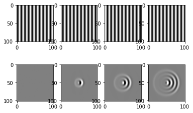
For $n=2$, $L=1$, $c=1$, with a single incident plane wave, $v_i(t,x) = \sin(\omega(t - \xi\cdot x))$, with direction $\xi$ and measurements parallel to the direction of propagation at the opposite end of the scattering potential. Use the Python code shown below to generate data for a given scattering potential, $r$.

Determine suitable $\Delta t$, $\Delta x$ and $T$ and generate data for scattering potential $u(x) = \exp(-200|x|^2)$ and an incident plane wave with $\xi = (1,0)$ and $\omega = 10\pi$.
Construct a non-scattering potential for this incident field and measurements by using the result you obtained in the previous exercise.
Can you construct a non-scattering potential that is invisible from multiple directions?

import numpy as np
import scipy.sparse as sp
import matplotlib.pyplot as plt

def solve(q,c,dt,dx,T=1.0,L=1.0,n=1):
	'''Solve n-dim wave equation using Leap-Frog scheme: u_{n+1} = Au_n + Bu_{n-1} + Cq_n'''
	# define some quantities
	gamma = dt*c/dx
	nt = int(T/dt + 1)
	nx = int(2*L/dx + 2)
	#
	q.resize((nx**n,nt))
	# define matrices
	A,B,C,L = getMatrices(gamma,nx,n)

	# main loop
	u = np.zeros((nx**n,nt))

	for k in range(1,nt-1):
		u[:,k+1] = A@u[:,k] + L@u[:,k] + B@u[:,k-1] + (dx**2)*C@q[:,k]

	return u

def multiply(u,c,dt,dx,T=1.0,L=1.0,n=1):
	# define some quantities
	gamma = dt*c/dx
	nt = int(T/dt + 1)
	nx = int(2*L/dx + 2)

	#
	u.resize((nx**2,nt))

	# define matrices
	A,B,C,L = getMatrices(gamma,nx,n)

	# main loop
	q = np.zeros((nx**n,nt))

	for k in range(1,nt-1):
		q[k] = (u[:,k+1] - 2*u[:,k] + u[:,k-1] - L@u[:,k])/(dt*c)**2

	return u

def sample(xin,xout1,xout2=[]):
	'''Spatial sampling by simple interpolation'''

	if len(xout2):
		n = 2
	else:
		n = 1

	m = len(xout1)
	nx = len(xin)

	rw = []
	cl = []
	nz = []

	if n == 1:
		for k in range(m):
			i = 0
			while xin[i] < xout1[k]:
				i = i + 1
			if i < nx - 1:
				a = (xout1[k] - xin[i+1])/(xin[i] - xin[i+1])
				b = (xout1[k] - xin[i])/(xin[i+1] - xin[i])
				rw.append(k)
				cl.append(i)
				nz.append(a)
				rw.append(k)
				cl.append(i+1)
				nz.append(b)
		P = sp.coo_matrix((nz,(rw,cl)),shape=(m,nx))
	else:
		for k in range(m):
			i = 0
			j = 0
			while xin[i] < xout1[k]:
				i = i + 1
			while xin[j] < xout2[k]:
				j = j + 1
			if i < nx - 1 and j < nx - 1:
				a = (xout1[k] - xin[i+1])*(xout2[k] - xin[j+1])/(xin[i] - xin[i+1])/(xin[j] - xin[j+1])
				b = (xout1[k] - xin[i])*(xout2[k] - xin[j+1])/(xin[i+1] - xin[i])/(xin[j] - xin[j+1])
				c = (xout1[k] - xin[i+1])*(xout2[k] - xin[j])/(xin[i] - xin[i+1])/(xin[j+1] - xin[j])
				d = (xout1[k] - xin[i])*(xout2[k] - xin[j])/(xin[i+1] - xin[i])/(xin[j+1] - xin[j])

				rw.append(k)
				cl.append(i+nx*j)
				nz.append(a)

				rw.append(k)
				cl.append(i+1+nx*j)
				nz.append(b)

				rw.append(k)
				cl.append(i+nx*(j+1))
				nz.append(c)

				rw.append(k)
				cl.append(i+1+nx*(j+1))
				nz.append(d)
		P = sp.coo_matrix((nz,(rw,cl)),shape=(m,nx*nx))

	return P

def getMatrices(gamma,nx,n):

# setup matrices
	l = (gamma**2)*np.ones((3,nx))
	l[1,:] = -2*(gamma**2)
	l[1,0] = -gamma
	l[2,0] = gamma
	l[0,nx-2] = gamma
	l[1,nx-1] = -gamma

	if n == 1:
		a = 2*np.ones(nx)
		a[0] = 1
		a[nx-1] = 1

		b = -np.ones(nx)
		b[0] = 0
		b[nx-1] = 0

		c = (gamma)**2*np.ones(nx)
		c[0] = 0
		c[nx-1] = 0

		L = sp.diags(l,[-1, 0, 1],shape=(nx,nx))

	else:
		a = 2*np.ones((nx,nx))
		a[0,:] = 1
		a[nx-1,:] = 1
		a[:,0] = 1
		a[:,nx-1] = 1
		a.resize(nx**2)

		b = -np.ones((nx,nx))
		b[0,:] = 0
		b[nx-1,:] = 0
		b[:,0] = 0
		b[:,nx-1] = 0
		b.resize(nx**2)

		c = (gamma)**2*np.ones((nx,nx))
		c[0,:] = 0
		c[nx-1,:] = 0
		c[:,0] = 0
		c[:,nx-1] = 0
		c.resize(nx**2)

		L = sp.kron(sp.diags(l,[-1, 0, 1],shape=(nx,nx)),sp.eye(nx)) + sp.kron(sp.eye(nx),sp.diags(l,[-1, 0, 1],shape=(nx,nx)))

	A = sp.diags(a)
	B = sp.diags(b)
	C = sp.diags(c)

	return A,B,C,L

# grid
nt = 201
nx = 101
x = np.linspace(-1,1,nx)
y = np.linspace(-1,1,nx)
t = np.linspace(0,1,nt)
xx,yy,tt = np.meshgrid(x,y,t)

# velocity
c = 1.0

# scattering potential
a = 200;
r = np.exp(-a*xx**2)*np.exp(-a*yy**2);

# incident field, plane wave at 10 Hz.
omega  = 2*np.pi*5
ui = np.sin(omega*(tt - (xx + 1)/c))

# solve
us = solve(r*ui,c,t[1]-t[0],x[1]-x[0],n=2)

# sample
xr = 0.8*np.ones(101)
yr = np.linspace(-1,1,101)

P = sample(x,xr,yr)

d = P@us

# plot
ui.resize((nx,nx,nt))
us.resize((nx,nx,nt))

plt.subplot(241)
plt.imshow(ui[:,:,1])
plt.clim((-1,1))

plt.subplot(242)
plt.imshow(ui[:,:,51])
plt.clim((-1,1))

plt.subplot(243)
plt.imshow(ui[:,:,101])
plt.clim((-1,1))

plt.subplot(244)
plt.imshow(ui[:,:,151])
plt.clim((-1,1))

plt.subplot(245)
plt.imshow(us[:,:,1])
plt.clim((-.001,.001))

plt.subplot(246)
plt.imshow(us[:,:,51])
plt.clim((-.001,.001))

plt.subplot(247)
plt.imshow(us[:,:,101])
plt.clim((-.001,.001))

plt.subplot(248)
plt.imshow(us[:,:,151])
plt.clim((-.001,.001))

plt.show()

9.5.2. Parameter estimation¶

For $n=1$, $c=1$, $L=1$, $q(t,x) = w''(t - t_0)\delta(x - x_0)$, with $t_0 = 0.2$, $x_0 = -0.5$ and where $w$ is given by $$ w(t) = \exp(-(t/\sigma)^2/2). $$

Express the solution $v(t,x)$ by using the Green function

The measurements are given by $f(t) = K(c) \equiv v(t,0.5)$. Consider retrieving the soundspeed $c$ by minimizing

\[ J(c) = \|K(c) - f\|^2. \]

Plot the objective as a function of $c$ for various values of $\sigma$.
Do you think Newton’s method will be successful in retrieving the correct $c$?

10 Lectures on Inverse Problems and Imaging

Wavefield Imaging

Contents

9. Wavefield Imaging¶

9.1. Forward modelling¶

9.1.1. Analytic solution¶

9.1.2. Numerical modelling¶

9.2. Analysis¶

9.2.1. Source localization¶

9.2.2. Inverse scattering¶

9.3. Reconstruction¶

9.3.1. Inverse source problem¶

9.3.2. Inverse scattering¶

9.3.3. Waveform tomography¶

9.4. Exercises¶

9.4.1. Inverse source problem¶

9.4.2. Inverse scattering¶

9.5. Assignments¶

9.5.1. Non-scattering potentials¶

9.5.2. Parameter estimation¶