
Given $m$ samples $x^{(i)} \in \mathbb{R}^n$, find a simple description / summary of the dataset.
- construct a probability distribution $f(x)$
- construct a reduced dataset $\widetilde{X} = UV^T$, with $U \in \mathbb{R}^{n\times p}$ and $V \in \mathbb{R}^{m\times p}$ that requires $\mathcal{O}(m + n)$ storage.
Density estimation
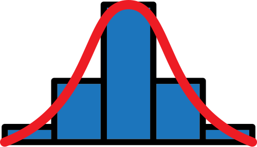
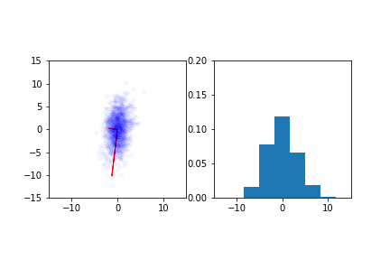
Example: Normal distribution
Fit a normal distribution to the samples
$$\max_{\mu,\Sigma} \prod_{i=1}^m(2\pi)^{-n/2}\text{det}(\Sigma)^{-1/2}\exp\left(-\frac{1}{2}(x^{(i)} - \mu)^T\Sigma^{-1}(x^{(i)} - \mu)\right)$$
leads to $$\min_{\mu,\Sigma}\,\, m\log(|\Sigma|) + \sum_{i=1}^m(x^{(i)} - \mu)^T\Sigma^{-1}(x^{(i)} - \mu)$$
which gives $$\widehat{\mu} = \frac{1}{m}\sum_{i=1}^m x^{(i)}, \quad \widehat{\Sigma} = \frac{1}{m}\sum_{i=1}^m \left(x^{(i)} - \widehat{\mu}\right)\left(x^{(i)} - \widehat{\mu}\right)^T.$$
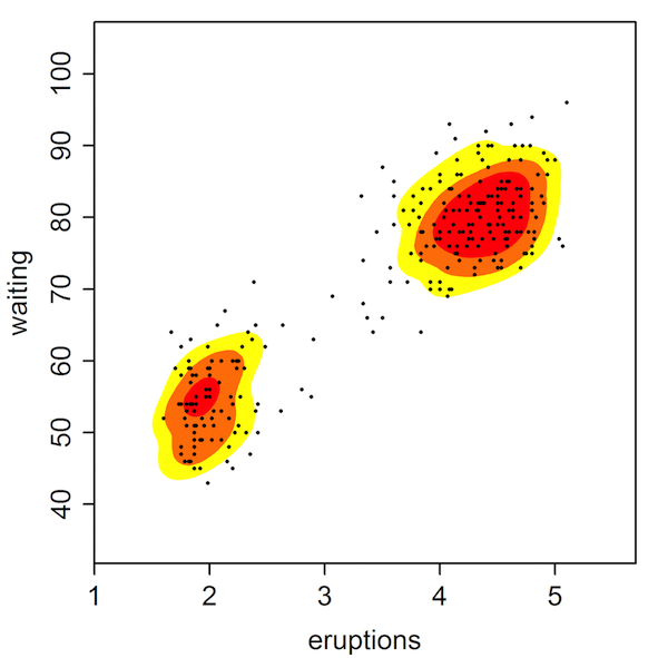
Example: Gaussian mixture model
Here, the goal is to fit a probability distribution of the form $$f(x) = \sum_{i=1}^k w_i f_i(x),$$ where $f_i(x)$ is a Normal distribution with paramaters $(\mu_i, \Sigma_i)$.
Can be obtained by solving $$\min_{\mu, \Sigma} -\log\left(\sum_{i=1}^k w_i f_i(x)\right).$$
Example: Sparse (inverse) covariance estimation
Given a sample-covariance matrix $C$, find an approximation, $\Sigma$, that has a sparse inverse:
$$\min_{\Sigma \succ 0} -\log|\Sigma| + \text{trace}(C\Sigma) + \alpha \|\Sigma\|_1.$$
- used to detect network structure in data
- large-scale algorithms available
- has a closed-form solution for very specific cases
Dimensionality reduction
Organize the data in a matrix $X = (x^{(1)}, x^{(2)}, \ldots, x^{(m)})$
- the matrix $C = XX^T$ is a sample-approximation of $\mathbb{E}(x_i x_j)$
- the matrix $C = X^TX$ gives information about the similarity or pairwise-distances between $x^{(i)}$ and $x^{(j)}$
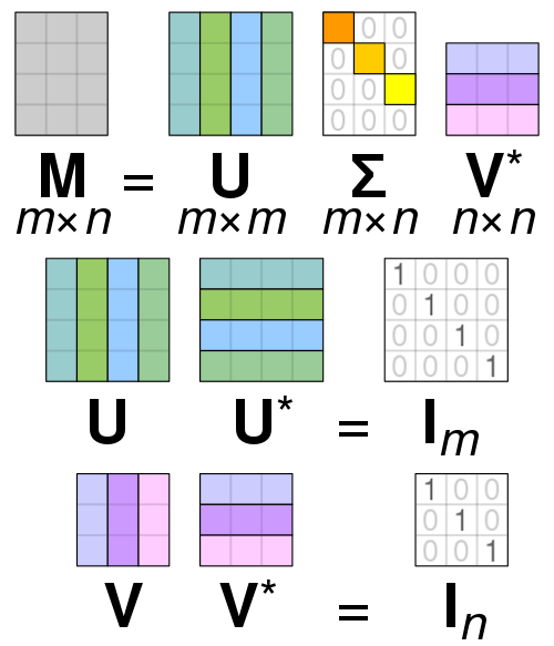
Singular value decomposition
A matrix $X \in \mathbb{R}^{n \times m}$ has a singular value decomposition $$X = U S V^T,$$ with $U \in \mathbb{R}^{n\times n}$, $V \in \mathbb{R}^{m\times m}$ are unitary matrices and $S$ is a diagonal matrix with non-negative entries.
- Expressing each column of $X$ (sample) as linear combination of the colums of $U$.
- Approximate the matrix by leaving out the unimportant components (small singular values)
$$X \approx \widetilde{X} = U_p S_p V_p^T.$$
- We can think of $\widetilde{X}$ as the solution of $$\min_{\widetilde{X}} \|X - \widetilde{X}\|_{F}^2 \quad \text{s.t.} \quad \text{rank}(\widetilde{X}) \leq p.$$
All together now!
- $$\left(\begin{matrix} 1 & 2 & 3 \\ 0 & 0 & 0 \end{matrix}\right)$$
- $$\left(\begin{matrix} 1 & 2 & 3 \\ 0 & 0 & 1 \end{matrix}\right)$$
- $$\left(\begin{matrix} 1 & 2 & 6 \\ 1 & 1 & 4 \\ 1 & 2 & 6 \end{matrix}\right)$$
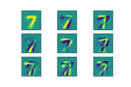
Example: Principle component analysis
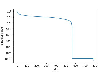
Singular values
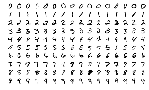
Example: Non-negative matrix factorization
Decompose a matrix in non-negative components
$$\min_{U,V} \|X - UV^T\|_{F}^2, \quad \text{s.t.} \quad u_{ij}, v_{ij} \geq 0$$
- used for clustering (when applied to $X^TX$)
- positivity is important for some applications (images)
Example: Robust PCA
$$\min_{\widetilde{X}} L(X - \widetilde{X}) \quad \text{s.t.} \quad \text{rank}(\widetilde{X}) \leq p,$$
where $L$ is a robust penalty (e.g., $L(R) = \|R\|_1$).
- Makes PCA less sensitive to outliers
- Applications in video-processing (low-rank + sparse)
Example: Matrix completion
Given partial knowledge of the entries of $X$, fill in the missing ones assuming a low-rank structure of $X$
$$\min_{W}\, \text{rank}(W) \quad \text{s.t.} \quad w_{ij} = x_{ij} \, \text{for}\, (i,j) \in \Omega.$$
- A famous example is the Netflix problem
![]()
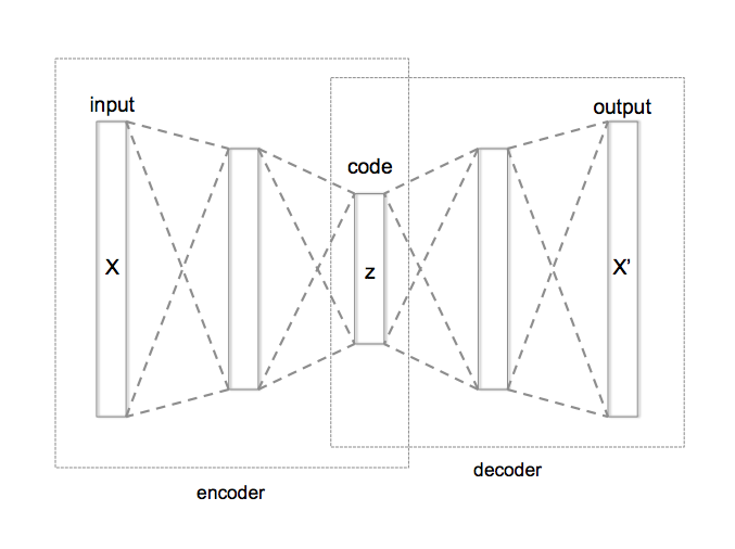
Example: Auto-encoders
- Find an encoder, $f$, and decoder, $g$ such that $x^{(i)} \approx g\circ f(x^{(i)})$ for all samples
- $z^{(i)} = f(x^{(i)})$ is the compressed sample
- Matrix factorization gives a linear encoder $f(x) = V^Tx$ and decoder $g(z) = Uz$.
- Popular auto-encoders are based on Neural Networks:
The story so far
Many problems in unsupervised learning involve
- the sample-covariance matrix $XX^T$ or similarity matrix $X^TX$
- an optimization problem with a matrix-valued unknown
- non-linear (e.g, $UV^T$) or non-convex (e.g. rank($W$)) terms
Challenges
- We may not be able to form matrices $XX^T$ and $X^TX$
- Computing the full SVD may not be computationally feasible
- We may have incomplete data
- Closed-form solutions may not be available
The rest of the talk
- Algorithms for approximating the SVD
- Optimization-based formulations
- Beyond matrices
Approximating the SVD
Goal is to decompose a matrix $$X = USV^T,$$ with $U$ and $V$ unitary and $S$ a non-negative diagonal matrix.
- The traditional approach has a computational complexity of $\mathcal{O}(mn^2)$ (when $m \geq n$).
- We usually only need a few of the largest singular vectors
Lanczos / Arnoldi method
Observation: repeated application of a matrix to a vector will align the vector with the largest eigenvector
- Start with a random vector $u_0$, compute $u_1 = (XX^T)^ku_0$, yields largest (left-) singular vector
- Repeat 1 starting from vector ortogonal to $u_1$, yielding $u_2$
- etc.
Randomized SVD
Observation: distances between points are preserverd under random projection (Johnson-Lindenstrauss Lemma).
There is a linear map $P \in \mathbb{R}^{k\times n}$ with $k > 8\log(m/\epsilon^2)$ such that $$(1 - \epsilon)\|x^{(i)} - x^{(j)}\|_2 \leq \|Px^{(i)} - Px^{(j)}\|_2 \leq (1 + \epsilon)\|x^{(i)}- x^{(j)}\|_2.$$
- Choose a suitable random matrix $P \in \mathbb{R}^{k\times n}$ with $k = \mathcal{O}(p)$
- Project all samples $x^{(i)}$ and collect in a matrix $Y \in \mathbb{R}^{k\times m}$
- Form an ortogonal basis, $Q$, for the row-space of $Y$
- Project the data matrix into a small matrix $B = XQ \in \mathbb{R}^{n \times k}$ perform an SVD on $B = U S \widetilde{V}^T$
- We get $X \approx U S \widetilde{V}Q^T$.
Comparison
Important factos when choosing a method are
- availability of the data (in core, out of core, streaming)
- required accuracy
- properties of the data (decay of singular values)
- need for parallelism
Optimization-based formulations
Both covariance estimation and matrix decomposition leads to optimization problems of the form
$$\min_{Z} \, L(Z) + R(Z),$$
- may include the constraint $Z \succ 0$ (positive definiteness).
- $R$ may be non-convex (e.g., $\text{rank}(Z)$)
- $L$ may be non-convex and non-smooth (e.g., $\text{nnz}(Z)$)
Basic ingredients
- manifold optimization
- convex relaxation
- coordinate descent
Manifold optimization
- encode structure ($Z \succ 0$, $\text{rank}(Z) = p$) explicitly
- this avoids non-convex or non-smooth penalties
- software libraries are available to help implement this (
Manopt,McTorch)
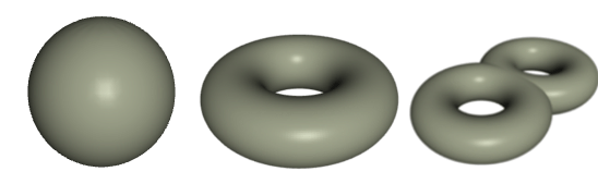
A Manifold
A Manifold
A Manifold
Manifold optimization
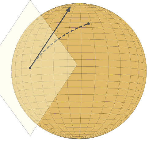
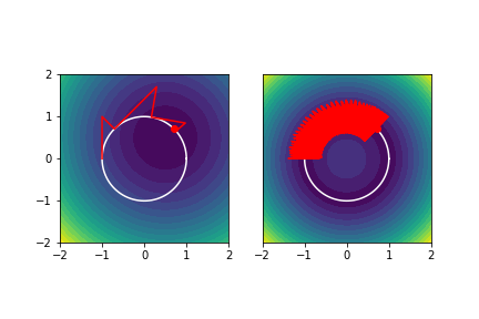
Simple example
$$\min_{x\in\mathbb{R}^2}\, f(x) \quad \text{s.t.} \quad \|x\|_2 = 1.$$
- Projection onto tangent space is given by $(I - xx^T)$, retraction by $\|x\|_2^{-1}I$.
- Using a penalty $|\|x\|_2 - 1|$ makes the problem non-convex
Symmetric positive definite matrices

Many of the programs discussed earlier can now be formulated as
$$\min_X\, L(X) + \alpha \|X\|_*,$$
where $\|X\|_*$ denotes the nuclear norm which is the sum of the singular values.
- Solution coincides with rank minimization in certain cases
- $\|X\|_*$ requires computing a singular value decomposition
- It may not be feasible to store the full matrix $X$
Non-convexification (?!)
- The nuclear norm may be written as an optimization problem $\|X\|_* = \min_{U,V} \textstyle{\frac{1}{2}}\left(\|U\|_F^2 + \|V\|_{F}^2\right) \quad \text{s.t.} \quad X = UV^T$.
- This suggests to formulate rank minimization as $$\min_{U,V}\, L(UV^T) + \frac{\alpha}{2}\left(\|U\|_F^2 + \|V\|_{F}^2\right).$$
- Solution coincides with nuclear norm minimization under certain circumstances
- Practical algorithms alternate between updating $U$ and $V$
Coordinate descent
Solve optimization problem $$\min_{Z} C(Z),$$ by updating one part of $Z$ at a time.
- one column: $$\min_{z} C(Z^{(k)} + ze_j^T),$$
- one row: $$\min_{z} C(Z^{(k)} + e_iz^T),$$
- one element: $$\min_{z} C(Z^{(k)} + ze_ie_j^T),$$
Coordinate descent
- Allows use of sophisticated optimization techniques
- Lot of heuristics available to select which blocks to update
- Asynchronous (parallel) variants are available as well
Tensors
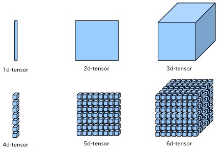
- Tensors can be used to capture higher order moments of the data ($\mathbb{E}(x_ix_jx_k\ldots)$)
- There are a number of ways to define an 'SVD' for tensors