

Overview
- From learning to Optimization
- Introduction to Optimization
- Some practical aspects
- Current trends
- From learning to Optimization
- Introduction to Optimization
- Some practical aspects
- Current trends
Supervised learning
Given samples $x^{(i)}$ and labels $y^{(i)}$ find a function $f$ such that $f(x^{(i)}) \approx y^{(i)}$
- For the purpose of this talk we'll consider $x^{(i)} \in \mathbb{R}^n$ and $y^{(i)} \in \mathbb{R}$ (regression) or $y^{(i)} \in \{-1,1\}$ (classification).
- Ultimately, one would use $f$ for prediction, so generalizability is very important. Today, we'll only discuss algorithms for finding $f$.
Fit a line through a set of points
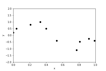
Fit a line through a set of points
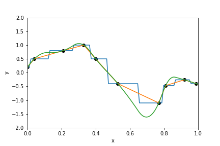
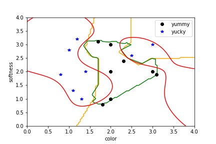
Figure out which papays are yummy
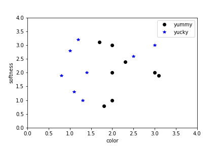
Figure out which papaya's are yummy
The supervised learning zoo
- Regression
- Neural networks
- Support Vector Machines
- ....
Example: Linear regression
$$f(x) = w_0 + \sum_{k=1}^n w_i x_i,$$
where the parameters are determined by solving
$$\min_{w} \sum_{i=1}^m \left(f(x_i) - y_i\right)^2$$
Example: binary classification
For classification $y_i \in \{-1,1\}$ we take
$$f(x) = \sigma\bigl(Wx + b\bigr),$$
with $\sigma(y) = (1 + \exp(-y))^{-1}$, and determine $w$ by solving
$$\min_{w} \sum_{i=1}^m \left(1 - y_if(x_i)\right)^2.$$
Example: Neural networks
$$f(x) = f_n \circ f_{n-1} \circ \ldots \circ f_1(x),$$ with $$f_k(x) = \sigma \left(W_k x + b_k\right).$$
- The architecture is determined by the structure of the matrices $W_k$.
- The optimal weights are found by training.
Example: Support vector machines
$$f(x) = \sum_{i=1}^m w_i k(x_i,x),$$
- The kernel $k(x,x')$ determines the properties of the function
- The weights are determined by solving $$\min_{w} L(f(x_i), y_i) + w^T\!Kw,$$ where $k_{ij} = k(x_i, x_j)$.
- From learning to Optimization
- Introduction to Optimization
- Some practical aspects
- Current trends
Optimization
Find a minimizer of a cost function $$C(w) = \sum_{i=1}^m L(f_i(w),y_i) + R(w),$$
where
- $w \in \mathbb{R}^n$ parametrizes the function
- $f_i(w)$ is the predicted label for $x_i$
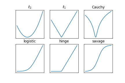
- $L(f(x),y)$ is the loss function, and
- $R(w)$ is the regularization term.
Example: linear regression
Let
- $f_i(w) = w_0 + \sum_{k=1}^n w_i x_i$
- $L(f_i,y_i) = (f_i - y_i)^2$
- $R(w) = \beta\|w\|_2^2$
This leads to a least-squares problem
$$C(w) = \|Xw - y\|_2^2 + \beta\|w\|_2^2,$$
with a closed-form solution
$$\widehat{w} = \left(X^T\!X + \beta I\right)^{-1}X^Ty.$$
Optimization
The optimization problem
$$\min_w \sum_{i=1}^m L(f_i(w),y_i) + R(w),$$
- Often does not have a closed-form solution
- May not have a unique minimizer
- Has too many variables to allow for sampling-based methods
- Does have a very particular structure
Furthermore:
- Evaluation of the cost function may be computationally expensive
- Evaluating the gradient may be difficult
- A good initial guess of the parameters may not be available
Optimization 101
- Structure of the cost function
- Optimality conditions
- Basic iterative algorithms
Structure of the cost function
Three properties come up frequently in optimization:
- Continuity
- Convexity
- Smoothness
Structure of the cost function - Lipschitz continuity
A function $C : \mathbb{R}^n \rightarrow \mathbb{R}$ is Lipschitz continuous with Lipschitz constant $\rho$ if $\forall \,w,w' \in \mathbb{R}^n$
$$\left|C(w) - C(w')\right| \leq \rho \|w - w'\|_2.$$
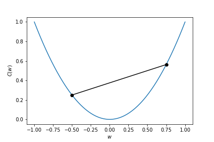
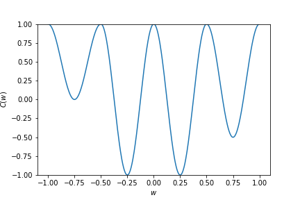
Structure of the cost function - convexity
A function $C : \mathbb{R}^n \rightarrow \mathbb{R}$ is convex if $\forall w,w' \in \mathbb{R}^n$ and $\forall t \in [0,1]$ we have
$$C(tw + (1-t)w') \leq tC(w) + (1-t)C(w').$$
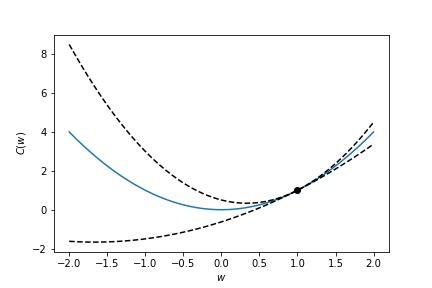
Structure of the cost function - smoothness
A function $C : \mathbb{R}^n \rightarrow \mathbb{R}$ is $\mathcal{C}^k$-smooth if all partial derivatives or order $\leq k$ exist and are continuous.
For $k \geq 1$:
- The Lipschitz constant can be found in terms of the gradient $\max_{w}\|\nabla C(w)\|$
- The Lipschitz constant of the gradient, $\ell$, is of interest.
- The function is $\mu$-strongly convex if $C(w) \geq C(w') + \langle \nabla C(w'),(w - w')\rangle + \frac{\mu}{2}\|w-w'\|_2^2$.
- The constant $\ell/\mu$ is called the condition number of $C$.
For $k \geq 2$:
- The Lipschitz constant of the gradient is the largest eigenvalue of the Hessian
- If the Hessian is positive semidefinite, the function is convex
- If the Hessian is positive definite, the function is strongly convex (with constant $\mu$ the smallest eigenvalue of the Hessian)
Structure of the cost function - strong convexity
Structure of the cost function
Note:
- It is often not possible to find the (global) bounds $(\ell, \mu)$ a-priori
- The objective may not be globally (strongly) convex, but is usefull to think of these as local properties that hold close to a minimizer
Optimality conditions - Local and global minima
- For convex functions, a local minimum is also a global minimum
- For strongly convex functions, the minimum is unique
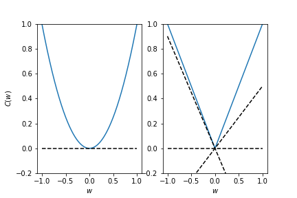
Optimality conditions (for local minima)
Smooth function:
- Gradient is zero, Hessian is positive (semi-)definite
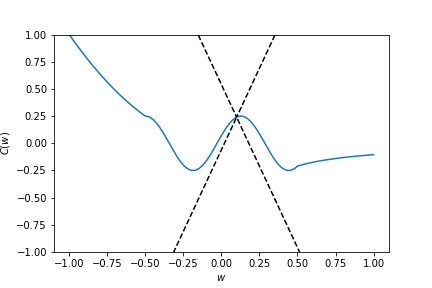
Convex function:
- Subgradient contains zero
Algorithms
Basic template (for smooth cost functions)
$$w_{k+1} = w_k + \alpha_k d_k,$$
where $\alpha_k$ is the stepsize and the search direction is constructed from the gradient:
- $d_k = - \nabla C(w_k)$ (steepest descent)
- $d_k = - \nabla C(w_k) + \beta_k d_{k-1}$ (conjugate gradients)
- $d_k = - B_k \nabla C(w_k)$ (quasi-Newton)
- $d_k = - \left(\nabla^2 C(w_k)\right)^{-1}\nabla C(w_k)$ (Newton's method)
Note that the search direction needs to be descent direction: $\langle \nabla C(w_k), d_k \rangle < 0$.
Algorithms - steepest descent
- for Lipschitz smooth $C$: $$\|\nabla C(w_k)\|^2 \leq c k^{-1}.$$
- for convex $C$ $$C(w_k) - C(w_*) \leq c k^{-1}.$$
- for strongly convex $C$: $$C(w_{k}) - C(w_*) \leq \left(1 - 2\mu\alpha_k + \mu\ell\alpha_k^2 \right)^{k}\left(C(w_0) - C(w_*)\right).$$
Algorithms - steepest descent
Steepest descent with a fixed stepsize ($\alpha_k \in (0,2/\ell)$):
The iterates converge to a stationary point from any initial point
For convex functions, the iterates converge to a minimum at a sub-linear rate of $\mathcal{O}(1/k)$
For strongly convex functions, the iterates converge to the minimum at a linear rate $\mathcal{O}(\rho^{k})$
To reach a point $w_k$ for which $|C(w_k) - C(w_*)| \leq \epsilon$ we need
- $\mathcal{O}(\epsilon^{-1})$ iterations with a sub-linear rate
- $\mathcal{O}(\log \epsilon^{-1})$ iterations with a linear rate
Algorithms - beyond steepest descent
- acceleration (conjugate gradient, momentum)
- second order methods (quasi-Newton, Gauss-Newton, Newton)
Algorithms - comparison
- Steepest descent: at best linear convergence to stationary point from any initial point
- Conjugate gradient / Quasi-newton: Faster convergence in practice (superlinear), less robust
- Full Newton: Quadratic convergence to local minimum when starting nearby
Algorithms - comparison
In practice we need to trade-off convergence rates, robustness and computational cost:
- Steepest descent has cheap iterations
- Quasi-Newton typically requires some storage to build up curvature information
- Full Newton requires the solution of a large system of linear equations at each iteration
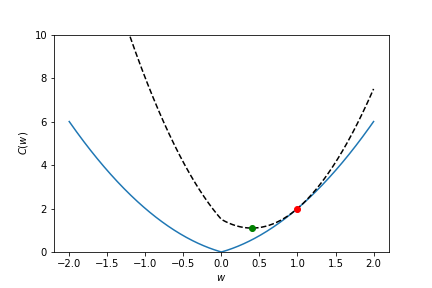
Algorithms for non-smooth regularization
We can use sub-gradients:
$$w_{k+1} = w_k - \alpha_k\left(\nabla L(w_k) + \partial R(w_k) \right),$$
and get a sub-linear convergence rate
...or modify the basic iteration to retain a linear convergence rate when $L$ is strongly convex
$$w_{k+1} = \mathrm{prox}_{\alpha_k R}\left(w_k - \alpha_k\nabla L(w_k)\right),$$
where $\text{prox}_{\alpha R}(z) = \text{argmin}_x \, R(x) + \frac{1}{2\alpha}\|z - x\|_2^2$.
Algorithms for non-smooth regularization
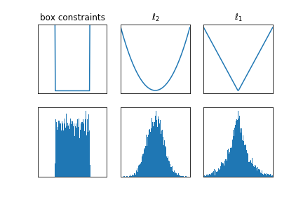
Note that when $R$ is the indicator of a convex set, the proximal operator projects onto the convex set.
- Box-constraints $w \in [-1,1]^n$: $\text{prox}(y) = \text{sign}(y)\cdot\min\{|y|,1\}$
- 2-norm ball $\|w\|_2 \leq \tau$: $\text{prox}(y) = \tau \cdot y / \|y\|_2$
- 1-norm ball $\|w\|_1 \leq \tau$: $\text{prox}(y) = \text{sign}(y)\cdot \max \{|y| - \tau, 0\}$
Other tricks of the trade
- Splitting techniques: $$\min_{w,v} C(w) + R(v) \quad \text{s.t.} \quad w = v,$$
- Smoothing/relaxation $$\min_{w,v} C(w) + R(v) + \frac{1}{2\epsilon}\|w - v\|_2^2,$$
- Partial minimization $$\min_{w_1,w_2} C(w_1,w_2) + R_1(w_1) + R_2(w_2)$$
- From learning to Optimization
- Introduction to Optimization
- Some practical aspects
- Current trends
Some practical issues
- Line search (learning rate)
- Bias-variance trade-off
- Level-set methods
- Vanishing/exploding gradient in RNN's
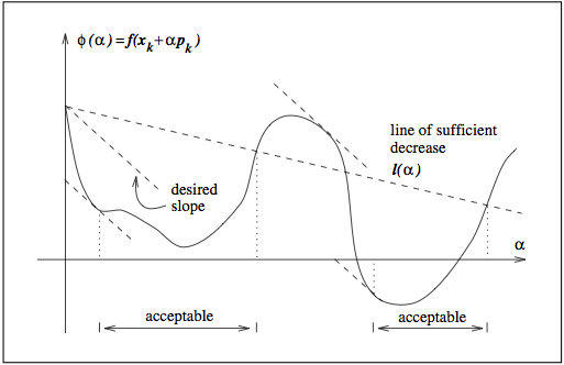
Line search
- Analysis so far was based on a constant (worst-case) stepsize.
- In practice, we can improve performance by choosing a clever stepsize.
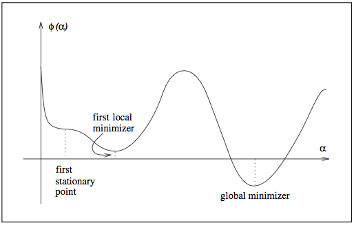
Sufficient decrease
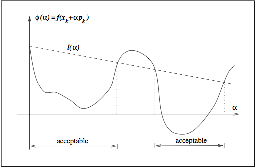
Curvature condition
Choosing an appropriate regularization parameter is its own optimization problem!
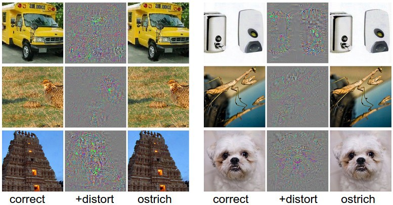
Ill-posedness
These examples indicate that the resulting $f$ is very sensitive;
$$|f(x) - f(y)| \leq C |x - y|,$$
for very large constant $C$.
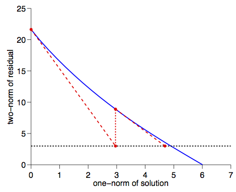
Level-set methods
When $C$ and $R$ are convex, the following three problems are equivalent
$$\min_{w} C(w) + \lambda R(w),$$
$$\min_{w} C(w) \quad \text{s.t.} \quad R(w) \leq \tau,$$
$$\min_{w} R(w) \quad \text{s.t.} \quad C(w) \leq \sigma.$$
- One formulation may be easier to solve then the other
- In terms of regularization, $\sigma$ or $\tau$ may be easier to estimate
The parameters $\tau$ and $\sigma$ are connected through the Pareto curve
To find the $\tau$ corresponding to a given $\sigma$ we solve a rootfinding problem with the value function
$$\phi(\tau) = \min_{w} C(w) \quad \text{s.t.} \quad R(w) \leq \tau.$$
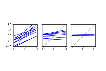
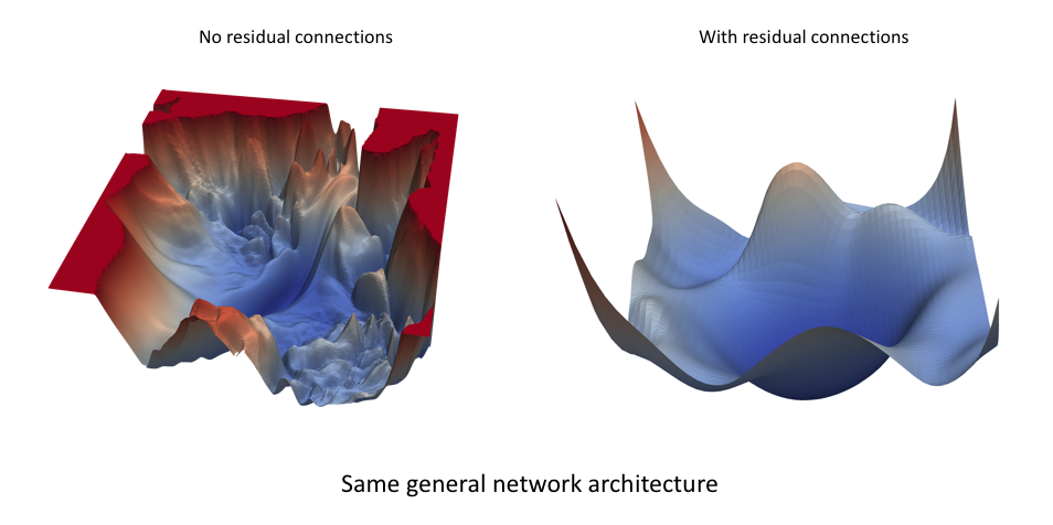
Vanishing / exploding gradients in RNN's
The function has a recursive structure: $$f(x_0) = x_n, \quad x_k = \sigma\left(W_{k-1} x_{k-1}+ b_{k-1}\right).$$
- Computing the gradient (back-propagation) requires evaluating the adjoint of the tangent linear model
$$\Delta x_{k} = \sigma'\left(W_{k-1} x_{k-1}+ b_{k-1}\right)\cdot (W_{k-1}\Delta x_{k-1}).$$
- This dynamical system may not be stable, even if the network is!
- The design of stable network architecturs is important in many deep-learning applications
- From learning to Optimization
- Introduction to Optimization
- Some practical aspects
- Current trends
Some current trends
- Stochastic optimization and acceleration
- Visualization/insight
- Modelling languages for optimization
We need to evaluate the objective at only one sample at a time: $$w_{k+1} = w_k - \alpha_k \nabla C(w_k; x_i),$$
or use a batch $$w_{k+1} = w_k - \frac{\alpha_k}{|\mathcal{I}_k|} \sum_{i\in\mathcal{I}_k}\nabla C(w_k; x_i)$$
We can interpret this algorithm as gradient-descent on the full objective that includes all $m$ training-samples with a noisy gradient: $\nabla C(w) + E_k$.
Batching
Full gradient: $$\nabla C(w) = \frac{1}{m}\sum_{i=1}^m \nabla C(w,x_i).$$
can be approximated using a sample-average $$\nabla C(w) \approx \frac{1}{|\mathcal{I}|}\sum_{i=\in\mathcal{I}} \nabla C(w,x_i)$$
Stochastic optimization
Main assumptions:
- $C$ is strongly convex
- Gradient direction is correct on average: $\mathbb{E}(E_k) = 0$ (e.g., choose $\mathcal{I}_k$ uniformly at random from $\{1, 2, \ldots, m\}$)
- Variance of the error is bounded: $\mathbb{E}(\|E_k\|_2^2)\leq \sigma^2$.
Basic iteration produces iterates for which $$\mathbb{E}(C(w_{k+1}) - C(w_*)) \leq \left(1 - 2\mu\alpha_k + \mu\ell\alpha_k^2\right)\left(C(w_{k}) - C(w_*)\right) + \frac{\alpha_k^2 \sigma ^2\ell }{2}.$$
$$\mathbb{E}(C(w_{k+1}) - C(w_*)) \leq \left(1 - 2\mu\alpha_k + \mu\ell\alpha_k^2\right)\left(C(w_{k}) - C(w_*)\right) + \frac{\alpha_k^2 \sigma ^2 \ell}{2}.$$
Stochastic optimization
We find
- linear convergence to a point close to a minimizer with fixed stepsize
- sublinear convergence to the minimizer when using a diminishing stepsize $\alpha_k = 1/k$.
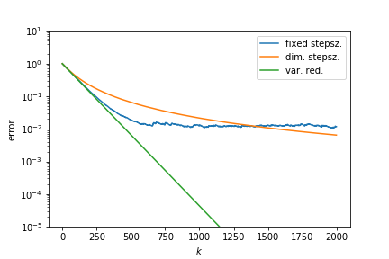
Acceleration
Linear convergence without stepsize reduction can be retained by variance reduction:
- Increase batchsize
- Use previous gradients (SVRG, SAGA)
Further improvements:
- Constants can be improved by gradient-scaling
- Accelaration for non-smooth terms using proximal algorithms
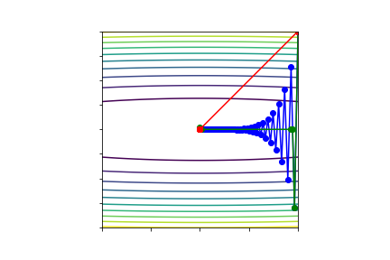
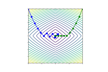
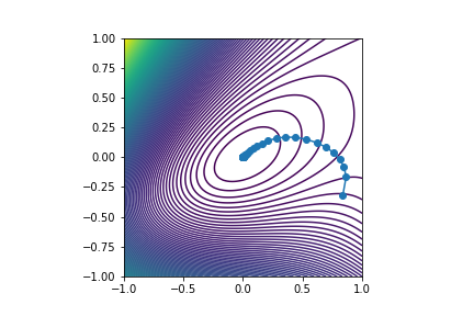
Visualization
Project iterates onto principal components of
$$M = \left(w_0 - w_n, w_{1} - w_{n}, \ldots, w_{n-1} - w_n\right),$$
and plot objective along dominant directions.
Modelling languages
Summary
- Supervised learning leads to interesting and structured optimization problems
- Many specialized algorithms are available to take advantage of this structure
- Stochastic methods can be usefully analyzed as gradient-descent-with-errors
- Exciting new research in (applied) math!