Lecture 4 - Filtered Back Projection

Contents

• The adjoint of the Radon transform
• Some usefull properties of the Radon transform
• Filtered back projection
• Assignments

The adjoint of the Radon transform

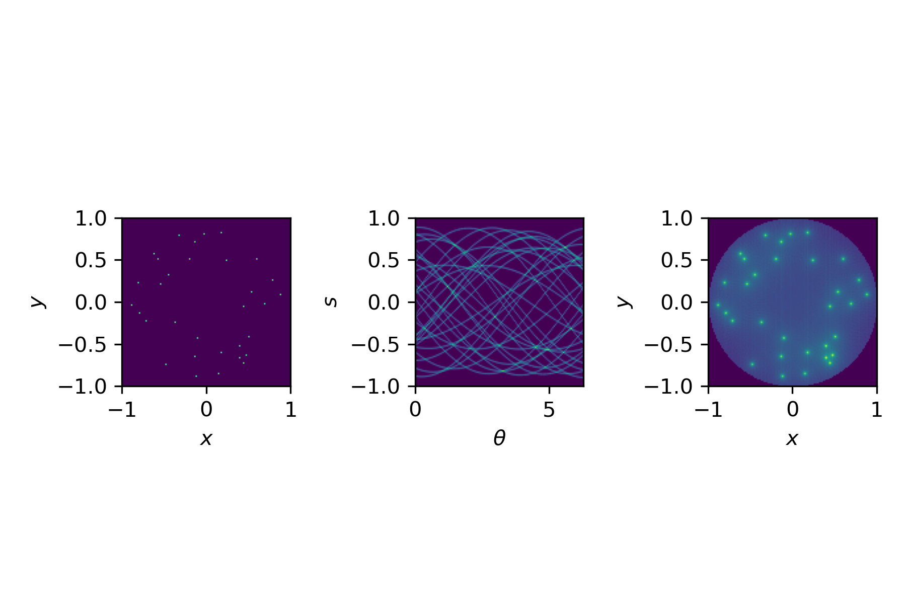
• The Radon transform integrates along lines
• The adjoint smears the sinogram back along these lines

It is defined as

$$u(\mathbf{x}) = \frac{1}{2\pi}\int_{0}^{2\pi} f(\mathbf{x}\cdot \mathbf{n}_\theta,\theta) \mathrm{d}\theta,$$

and is equivalent to the transpose of the mastrix in the discrete setting.

Some useful properties of the Radon transform

The second derivatices in $\mathbf{x}$ and $s$ intertwine with the Radon transform as follows

$$R \Delta_\mathbf{x} u = \partial_s^2 R u, $$

and

$$R^* \partial_s^2 f = \Delta_\mathbf{x} R^*f.$$

Furthermore

$$R^*\!R u = 2 \cdot (-\Delta_{\mathbf{x}})^{-1/2}u,$$

and

$$RR^* f = 2 \cdot (-\partial_s^2)^{-1/2} f.$$

This suggests we can invert the Radon transform via backprojection followed by 2D-filtering

$$u = \textstyle{\frac{1}{2}} \cdot (-\Delta_{\mathbf{x}})^{1/2} R^*f,$$

or 1D-filtering followed by backprojection

$$u = \textstyle{\frac{1}{2}} \cdot R^* (-\partial_s^2)^{1/2} f$$

Filtered back projection

(Courtesy of Samuli Siltanen)

The filter is naturally defined through the Fourier transform as it is equivelant to multiplying by $|\sigma|$ in the Fourier domain.

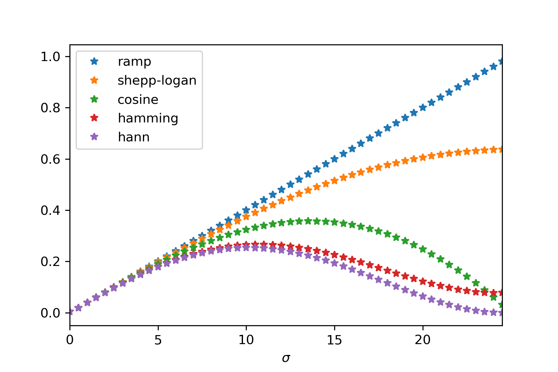
Here the filters are defined as (based on $\sigma \in [-1,1]$)

$$w(\sigma) = \begin{cases} |\sigma| & (\text{ramp}) \\ |(2/\pi)\sin(\pi \sigma / 2)| &(\text{Shepp-Logan}) \\ |\sigma \cos(\pi \sigma / 2)| & (\text{Cosine})\end{cases}$$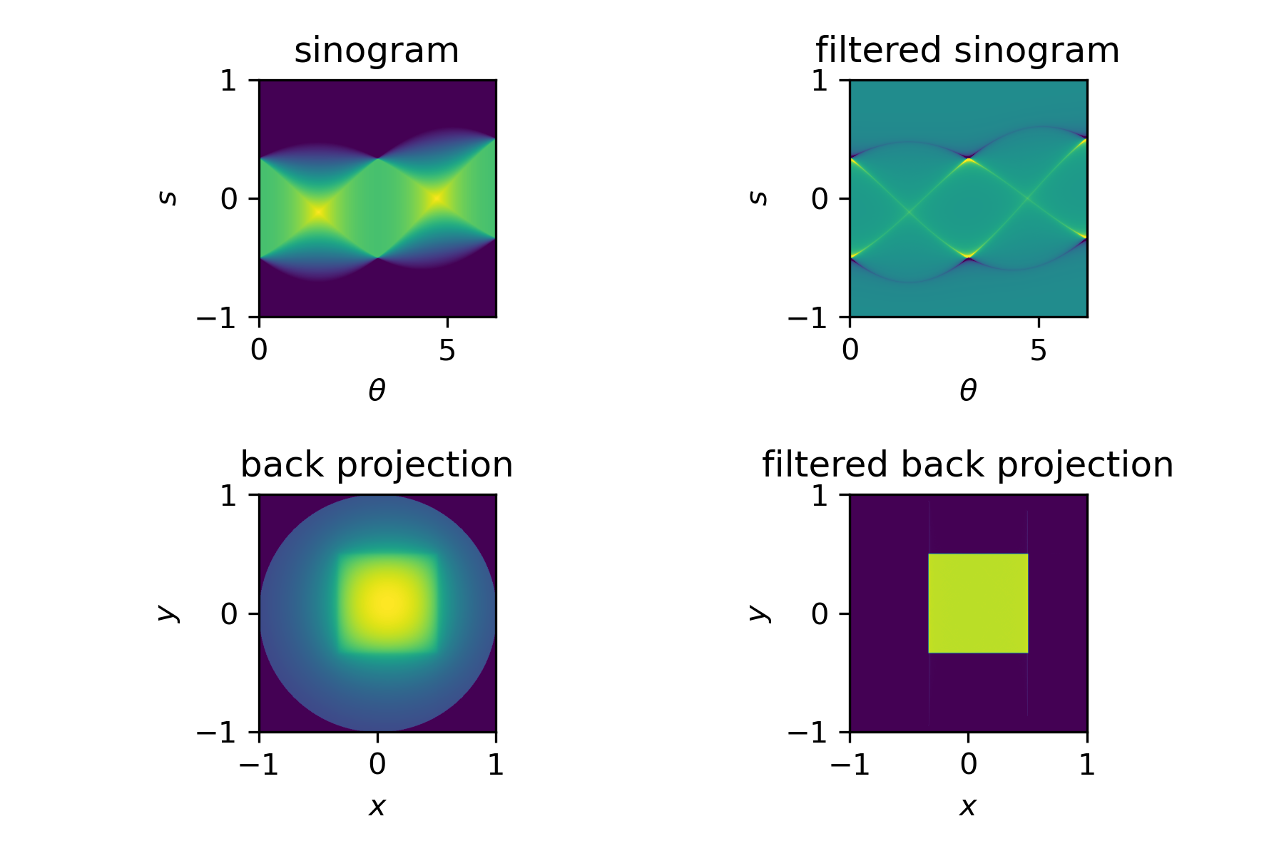

Assignments

Assignment 1

Implement filtered back projection for various filters and test its performance on noisy data.