Lecture 3 - Discretisation of the Radon Transform
Contents
- The discrete Radon transform
- Sparse matrices
- Matrix-free implementation
- Assignments
The Discrete Radon Transform
The Radon transform is defined as
$$f(\theta,s) = \int_{-\infty}^\infty u\left(x(s,t), y(s,t)\right) \mathrm{d}t,$$with
$$x(s,t) = t \sin \theta + s \cos \theta, \quad y(s,t) = t\cos\theta - s \sin \theta.$$- Let $s \in [-1,1]$ and discretise the detector in $n_d$ cells with width $2/n_d$.
- Let $(x,y) \in [-1,1]^2$ and discretise the image in $n_x \times n_y$ pixels with size $2/n_x \times 2/n_y$.
- Define basis functions $\phi_j(x,y)$ that are supported on the $j-th$ pixel.
- The contribution of the $j-th$ pixel to the $i-th$ detector element at angle $\theta$ is then given by
- The measurement along a single angle then leads to a matrix $A(\theta) \in \mathbb{R}^{n_d \times n_x \cdot n_y}$
We can now easily compute the matrix elements for a given set of angles $\{\theta_k\}_{k=1}^{n_\theta}$ and define
$$A = \left( \begin{matrix} A(\theta_1) \\ A(\theta_2) \\ \vdots \\ A(\theta_k)\end{matrix}\right).$$The vectorised discretised sinogram and image are then related via
$$\mathbf{f} = A\mathbf{u}.$$The line model
- The weights $a_{ij}$ represent the length of the intersection between the $j-th$ ray and the $i-th$ pixel.
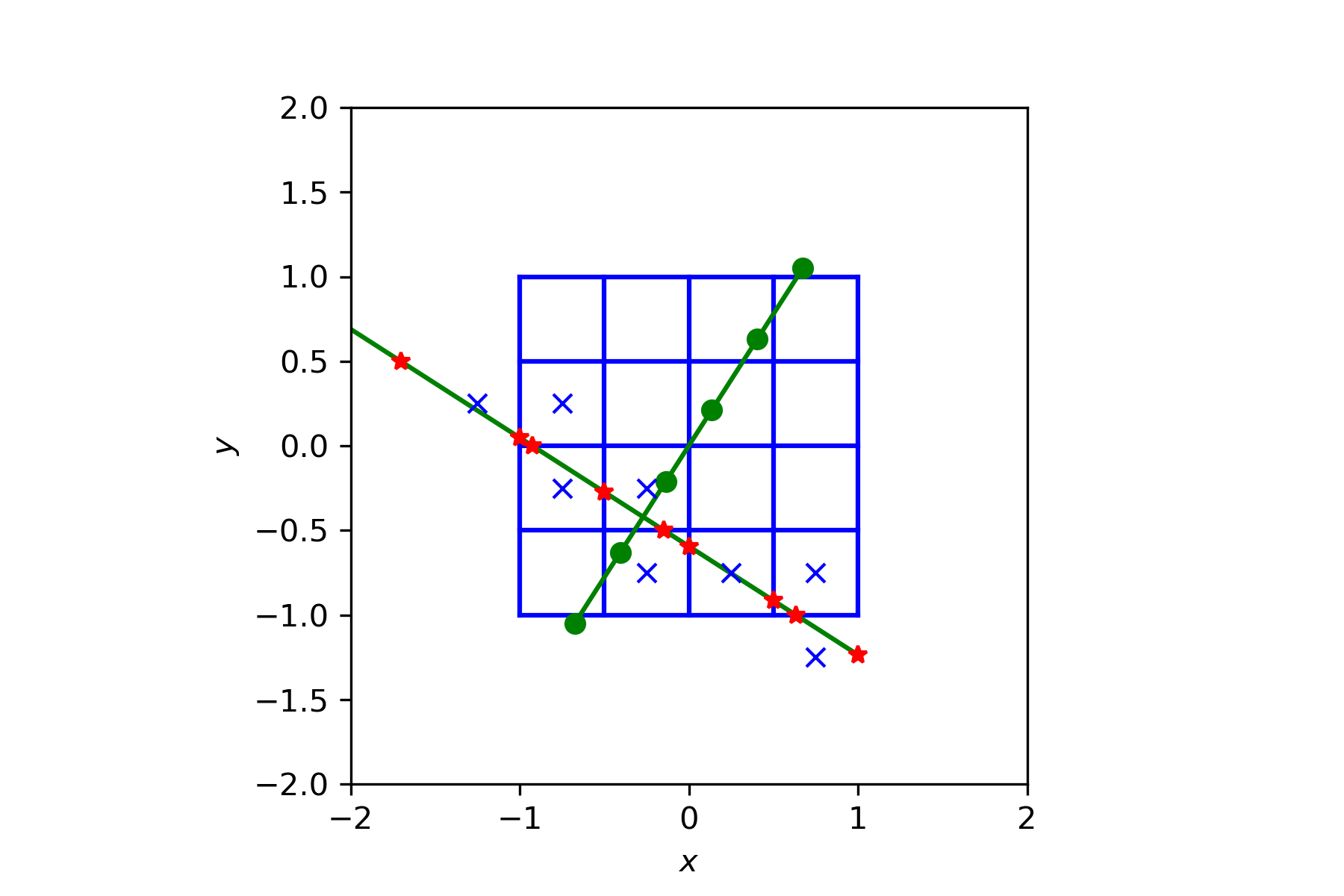
- We can compute these efficiently by solving for $t$ from $$x = t \sin \theta + s \cos \theta, \quad y = t\cos\theta - s \sin \theta,$$ where $s$ is given and $x,y$ are the grid lines.
- This yields an array of intersection points $\{t_k\}_k$ along the ray and $t_{k} - t_{k-1}$ gives the intersection length
- Substituting $(t_{k} + t_{k-1})/2$ back in the line equation and rounding yields the central coordinates of the intersected pixels
- We can use these to compute the indices $i$ of the pixels that are intersected by the $j-th$ ray
import numpy as np

x = np.array([-1, -.5, 0, .5, 1])
y = np.array([-1, -.5, 0, .5, 1])
h = 0.5
s = np.array([-1.25, -.75, -.25, .25, .75, 1.25])

theta = 1
si = -.5

tx = (x - si*np.cos(theta)) / np.sin(theta)
ty = -(y - si*np.sin(theta)) / np.cos(theta)
t  = np.sort(np.concatenate((tx,ty)))

xi = si*np.cos(theta) + t*np.sin(theta)
yi = si*np.sin(theta) - t*np.cos(theta)

xc = h*((si*np.cos(theta) + 0.5*(t[0:-1]+t[1:])*np.sin(theta))//h) + h/2
yc = h*((si*np.sin(theta) - 0.5*(t[0:-1]+t[1:])*np.cos(theta))//h) + h/2
Sparse matrices
- Let $n_x = n_y = n$ and $n_d = n_\theta = n$.
- We can easily see that we only have $\mathcal{O}(n)$ non-zeros in each row of the matrix; so $\mathcal{O}(n^3)$ non-zeros in total
- It is not very attractive to store and compute with all the zero-entries explicitly
Sparse matrix formats
coo_arrayCoordinate formatcsc_arrayCompressed Sparse Column formatcsr_arrayCompressed Sparse Row format
COO
CSC
CSR
Matrix-free implementation
- For 3D applications, we'd end up with a matrix with $\mathcal{O}(n^4)$ non-zeros
- Using double precision, storage may take several Terabytes in practice ($n = 1000$).
- Can we instead compute the matrix elements on-the-fly?
- We can write a function to perform multiplication of $A$ by a given vector implicitly
- This avoids storage, but may induce some computational overhead
- We cannot access individual elements of the matrix easily
- We need to write a seperate function to multiply with the transpose of the matrix
An example
Consider a finite-difference matrix
$$A = \left(\begin{matrix}-2 & 1& 0 & \ldots & \\ 1 & -2 & 1 & 0 \\ & \ddots & \ddots & \ddots & \\ 0 & \ldots &0 & 1 & -2 \end{matrix}\right).$$The function would look like
def FD(u, n):
    v       = np.zeros(n)
    v[0]    = -2*u[0] + u[1]
    v[1:-1] = u[:-2] - 2*u[1:-1] + u[2:]
    v[-1]   = u[-2] - 2*u[-1]
Another example
Consider summing the elements of a vector
$$A = (1, 1, 1, \ldots, 1).$$def sum(u,n):
return np.sum(u)
def sum_transpose(v,n):
    u = v * np.ones(n)
Assignments
Assignment 1
Write a function RadonMatrix(n, s, theta) that discretizes the Radon transform of a given n $\times$ n image, defined on $[-1,1]^2$, for given arrays s and theta and returns a matrix of size len(s)*len(theta) by n*n.
You can start with a loop that traces each ray individually and computes the weights in the matrix according to the procedure we outlined in class. If you are familiar with numpy you can attempt to make it more efficient.
Assignment 2
Write a function RadonSparseMatrix which returns a sparse matrix representation of RadonMatrix.
- Check that it indeed gives the same ouput as
RadonMatrix - Do you notice a difference in computational time for dense and sparse matrices?
- Check the above for multiplication with the matrix and its tranpose for various sparse matrix formats
Assignment 3
Write a function Radon(u, n, s, theta) which performs the Radon transform of the given image u and the corresponding transpose RadonTranspose(f, n, s, theta).
- Check that they give the same result as multiplying by the matrix
- Check the computational time and memory requirements