Lecture 2 - Fourier reconstruction

Contents

• The Fourier transform
• The Fourier-Slice Theorem
• Fourier reconstruction
• Assignments

The Fourier transform

The Fourier transform of a function $g : \mathbb{R} \rightarrow \mathbb{R}$ is given by

$$\widehat{g}(\xi) = \int_{\mathbb{R}} g(x) e^{-2\pi\imath x \xi} \mathrm{d}x.$$

The inverse transform is given by

$$g(x) = \int_{\mathbb{R}} \widehat{g}(\xi) e^{2\pi\imath x \xi} \mathrm{d}\xi.$$

Similarly, for a function $g : \mathbb{R}^n \rightarrow \mathbb{R}$

$$\widehat{g}(\boldsymbol{\xi}) = \int_{\mathbb{R}^n} g(\mathbf{x}) e^{-2\pi\imath x \cdot \boldsymbol{\xi}} \mathrm{d}\mathbf{x}.$$

With inverse

$$g(\mathbf{x}) = \int_{\mathbb{R}^n} \widehat{g}(\boldsymbol{\xi}) e^{2\pi\imath x \cdot \boldsymbol{\xi}} \mathrm{d}\boldsymbol{\xi}.$$

The Fourier-Slice Theorem

The Fourier-Slice Theorem relates the 2D-Fourier transform of $u$ to the 1D-Fourier transform of $f$:

$$\widehat{f}(\theta, \sigma) = \widehat{u}(\sigma \mathbf{n}_\theta),$$

with

$$\widehat{f}(\theta,\sigma) = \int_{\mathbb{R}} f(\theta,s) e^{-2\pi\imath \sigma s}\mathrm{d}s,$$$$\widehat{u}(\mathbf{k}) = \int_{\mathbb{R}^2} u(\mathbf{x}) e^{-2\pi\imath \mathbf{k}\cdot \mathbf{x}}\mathrm{d}\mathbf{x},$$$$\mathbf{n}_\theta = (\cos\theta,-\sin\theta).$$

We can visualise this as follows

Fourier reconstruction

• In principle, we can reconstruct the image by performing an inverse Fourier transform
• Having collected discrete measurements $f_{ij} = f(\theta_j,s_i)$, we only have partial information on the Fourier transform of $u$
• Ultimately, we will represent $u$ on a grid of pixels with intenties $u_i = u(\mathbf{x}_i)$

The Discrete Fourier Transform

The discrete Fourier transform (DFT) of a sequence $\{g_i\}_{i=0}^n$ is defined as

$$\widehat{g}_i = \sum_{j=0}^{n-1} g_j \exp\left(-\frac{2\pi\imath}{n} ij\right), \quad i = 0, \ldots, n-1.$$

When $g_i$ samples $g$ at a grid with spacing $\Delta x$, its Fourier spectrum $\widehat{g}$ is sampled with $\Delta \xi = (n\Delta x)^{-1}$.

We need to be carefull when trying to relate the samples $g_i, \widehat{g}_i$ to the underlying functions $g, \widehat{g}$.

• DFT assumes grids to be order as $(0, h, 2h, \ldots, L, L, L-h, \ldots, -h)$.
• Use fftshift and ifftshift to switch between DFT and normal ordering of the grid.

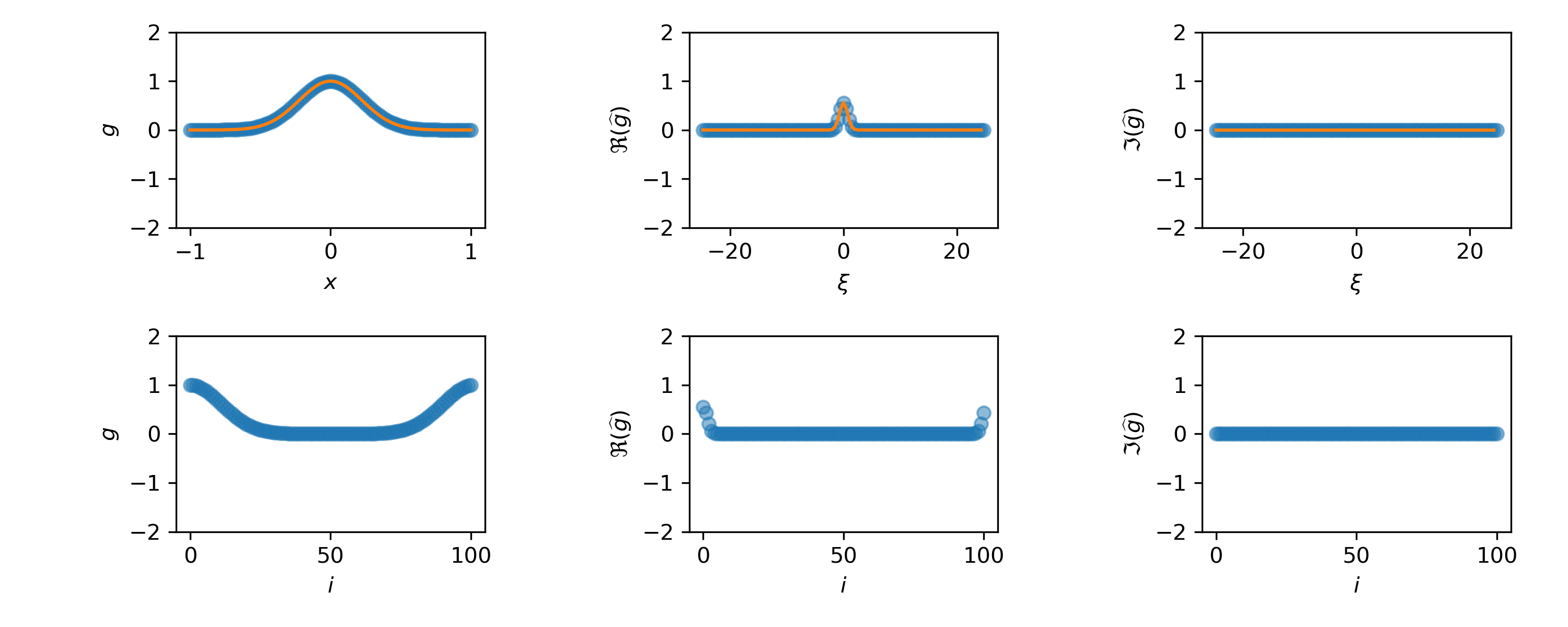
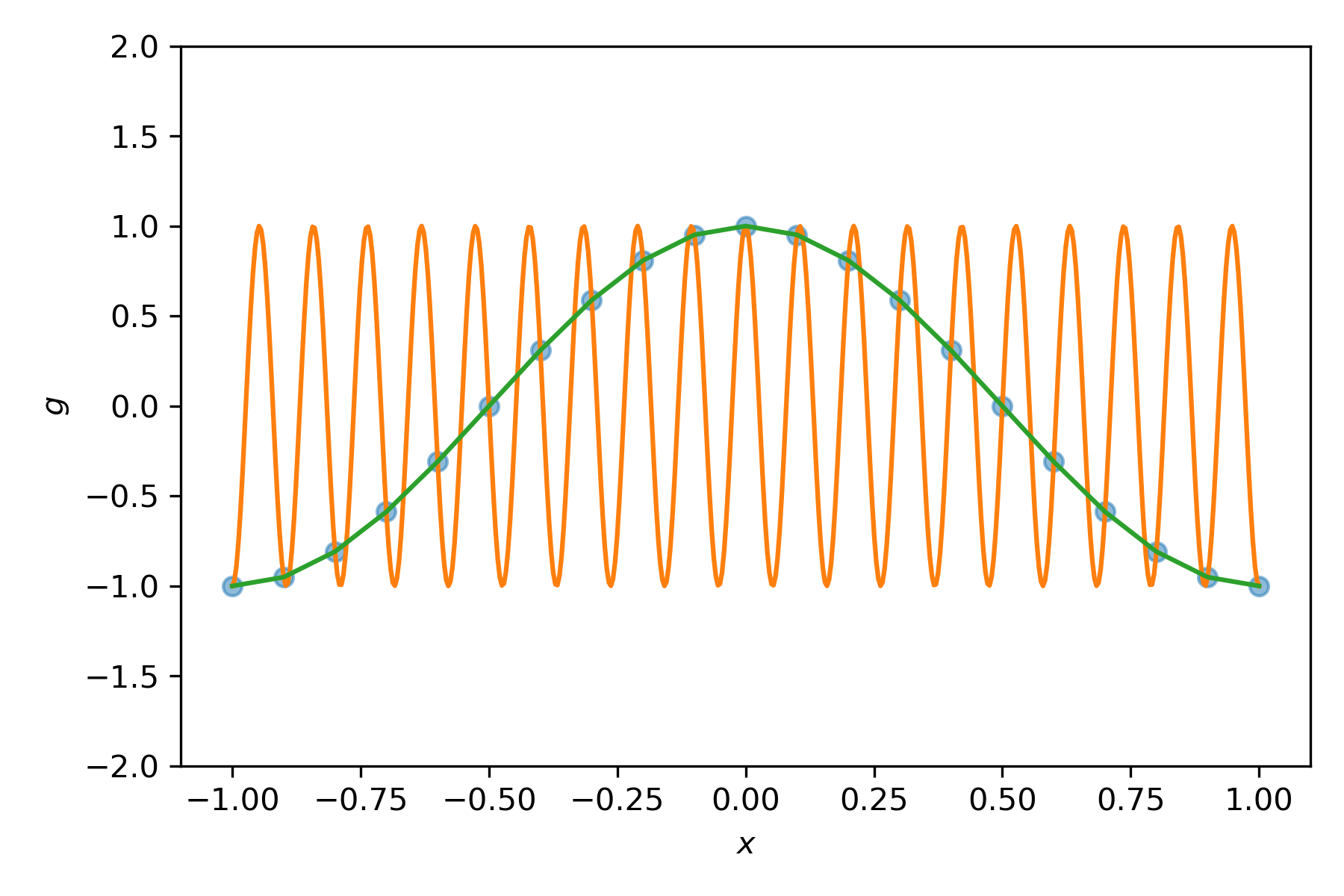
Be aware that some interesting things may happen with the DFT, when subsampling or truncating the signals.

The Fast Fourier Transform

A naive implementation would require $\mathcal{O}(n^2)$ operations to multiply by $F$. With some clever tricks, however, it can be done in $\mathcal{O}(n\log n)$.

To illustrate the concept, consider $n = 2^p$ and express the DFT as

$$\sum_{j=0}^{n-1} g_j \exp\left(-\frac{2\pi\imath}{n} ij\right) = \sum_{j=0}^{n/2-1} g_{2j} \exp\left(-\frac{2\pi\imath}{n} i(2j)\right) + \sum_{j=0}^{n/2-1} g_{2j+1} \exp\left(-\frac{2\pi\imath}{n} i(2j+1)\right)$$$$ = \underbrace{\sum_{j=0}^{n/2-1} g_{2j} \exp\left(-\frac{2\pi\imath}{n/2} ij\right)}_{E_i} + \exp\left(-\frac{2\pi\imath}{n} i\right)\underbrace{\sum_{j=0}^{n/2-1} g_{2j+1} \exp\left(-\frac{2\pi\imath}{n/2} ij\right)}_{O_i}$$

We need only compute $E_i$ and $O_i$ for $i = 0, \ldots, n/2-1$ since

$$\widehat{g}_i = E_i + e^{-\frac{2\pi\imath}{n} i} O_i, \quad \widehat{g}_{i+n/2} = E_i - e^{-\frac{2\pi\imath}{n} i} O_i$$

This divide-and-conquer technique leads to an overall complexity of $\mathcal{O}(n\log n)$.

Interpolation

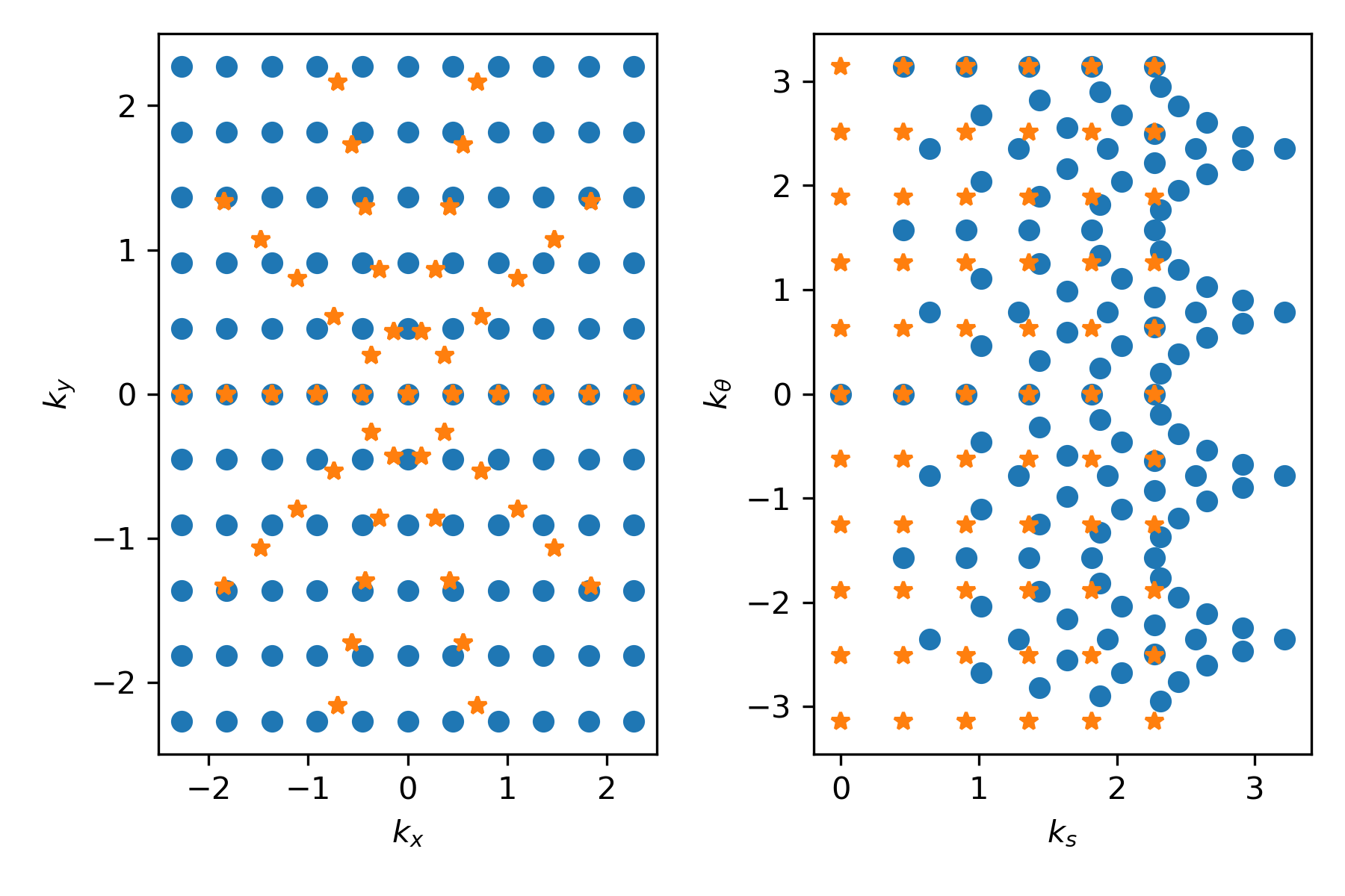
Applying the Fourier transform to $f_{ij}$ gives us samples of $\widehat{u}$ at wavenumbers

$$\{(\sigma_i \mathbf{n}_{\theta_j})\},$$

with $\sigma_i = i \cdot (n h)^{-1}$ for $i = -(n-1)/2, \ldots, 0, \ldots, (n-1)/2$ (assuming again that $f_{ij} = f(i \cdot h , \theta_j)$ and $n$ odd)

To usefully apply the inverse DFT, we need $\widehat{u}$ at wavenumbers

$$\{(i\cdot (n h)^{-1}, j\cdot (n h )^{-1})\},$$

for $i,j = -(n-1)/2, \ldots, 0, \ldots, (n-1)/2$.

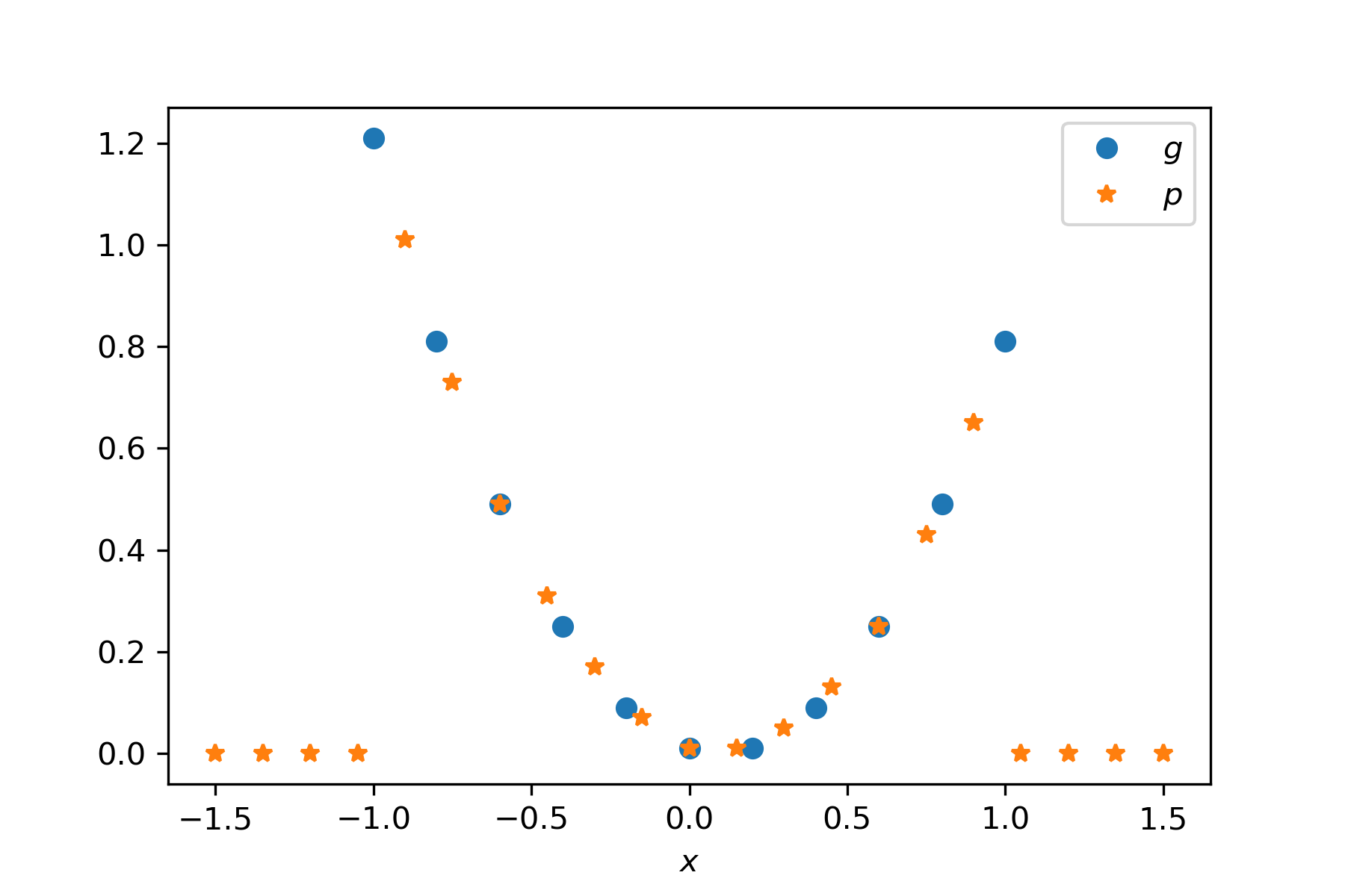
In interpolation we aim to approximate the value of a function $g$ at $(x,y)$ from its values at nearby points $g_i = g(x_i,y_i)$.

• Linear interpolation uses 3 nearby points
• Bi-linear interplation uses 4 nearby points

For linear interpolation, we use a first order polynomial of the form

$$p(x,y) = a \cdot x + b \cdot y + c,$$

and set up a system of equations for $(a,b,c)$ by demanding that $p(x_i,y_i) = g_i$.

For bi-linear interpolation, we use a polynomial of the form

$$p(x,y) = a \cdot x \cdot y + b \cdot x + c \cdot y + d,$$

and set up a system of equations for $(a,b,c,d)$ by demanding that $p(x_i,y_i) = g_i$.

1D example

def lininterp1d(x,g,xs):
    """
    Linear interpolation from regular grid.

    x  - input grid (regularly spaced), 1d array of length n
    g  - function values, 1d array of length n
    xs - values at which to evaluate, 1d array of length ns
    """

    n = len(x)
    ns = len(xs)
    gs = np.zeros(ns)

    h = x[1] - x[0]

    for i in range(ns):
        j = int((xs[i] - x[0]) // h) # find j such that x[j] <= xs[i] < x[j+1]
        if 0 <= j < n-1:
            gs[i] = ((x[j+1] - xs[i])/h)*g[j] + ((xs[i] - x[j])/h)*g[j+1]
        else:
            gs[i] = 0

    return gs

Assignments

Assignment 1

Implement a function to bi-linearly interpolate data from a polar grid r,theta to a cartesian grid x,y. Use the following template

def interpolate(f_hat, theta, ks, kx, ky):
    """
    Bi-linear interpolation from radial grid (ks,theta) to cartesian grid (kx,ky), 
    related via kx = ks*cos(theta), ky = -ks*sin(theta).

    The radial coordinates are assumed to include negative radii and theta \in [0,pi).

    Input: 
        f_hat     - 2d array of size (ns,ntheta) containing values on the radial grid
        theta, ks - 1d arrays of size ns and nt containing the polar gridpoints
        kx, ky    - 1d arrays of size nx and ny containing the cartesian gridpoints

    Output:
        u_hat     - 2d array of size (nx,nt) containing the interpolated values
    """

Assignment 2

Use your interpolation method to reconstruct the following data

# settings
nx = 400
na = 400
theta = np.linspace(0., 180., na)
sigma = 1

# phantom
u = shepp_logan_phantom()

# sinogram
f = radon(u, theta=theta)
f_noisy = f + sigma * np.random.randn(nx,na)

• perform a one-dimensional fft of the sinogram; you can use fftshift and ifftshift to switch between the regular and DFT ordering of grid.
• define the corresponding polar Fourier grid (according to the Fourier Slice Theorem)
• interpolate the data on a euclidian grid
• Vary the noise level sigma and angular sampling na; is Fourier reconstruction more or less sensitive to noise and subsampling than iradon?