Lecture 1 - What is Computed Tomography
Contents
- A bit of history
- Physics of X-rays
- The Radon Transform
- Computed Tomography
- Assignments
A bit of History
X-rays were accidentally discovered in 1895 by Wilhelm Röntgen

The first published X-ray photograph of the hand of Anna Bertha Ludwig (Röntgen's wife)

- X-ray photography was soon adopted for medical use and even recreational use
- The potential dangers of prolonged exposure to X-rays was not recognized untill much later
- X-ray photography is still an important tool for medical diagnosis
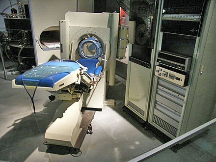
The first prototype CT scanner was built in 1961 by William Oldendorf

The first commercial scanner, developed by Godfrey Hounsfield, became available in 1971. A scan took 5 minutes, and processing the data took around 2.5 hours.
The mathematics behind tomography was developed partially independent of scanning technology
- 1917: Johan Radon described a method for reconstruction a function from its line integrals
- 1937: Stefan Kaczmarz developed a method to find an approximate solution to a large system of linear algebraic equations
- 1963-1964: Allan MacLeod Cormack published 2 landmark papers on tomographic image reconstruction
Computed Tomography is still an active area of research in Mathematics.
The Physics of X-rays
When passing through an object, an X-ray beam loses intensity through absorption and scattering. This process can be approximately described by the Beer-Lambert law:
$$I = I_0 \exp^{-\mu h},$$where
- $I_0$ is the intensity of the incoming X-ray beam
- $I$ is the intensity of the outgoing X-ray beam
- $\mu$ is the linear attenuation coefficient of the material
- $h$ is the thickness of the material
If the X-ray passes through multiple materials, we have
$$I = I_0 \exp\left(-\sum_i \mu_i h_i\right),$$which in the limit becomes
$$I = I_0 \exp\left(-\int \mu(t) \mathrm{d}t\right).$$We can transform this to a linear relation between measured and unknown quantities:
$$-\log\left(I / I_0\right) = \int \mu(t) \mathrm{d}t.$$The Radon Transform
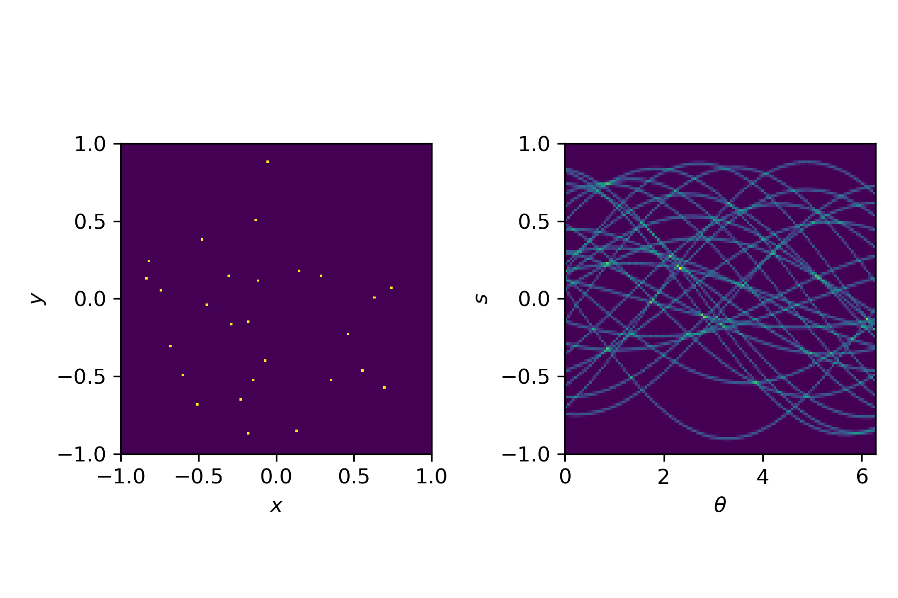
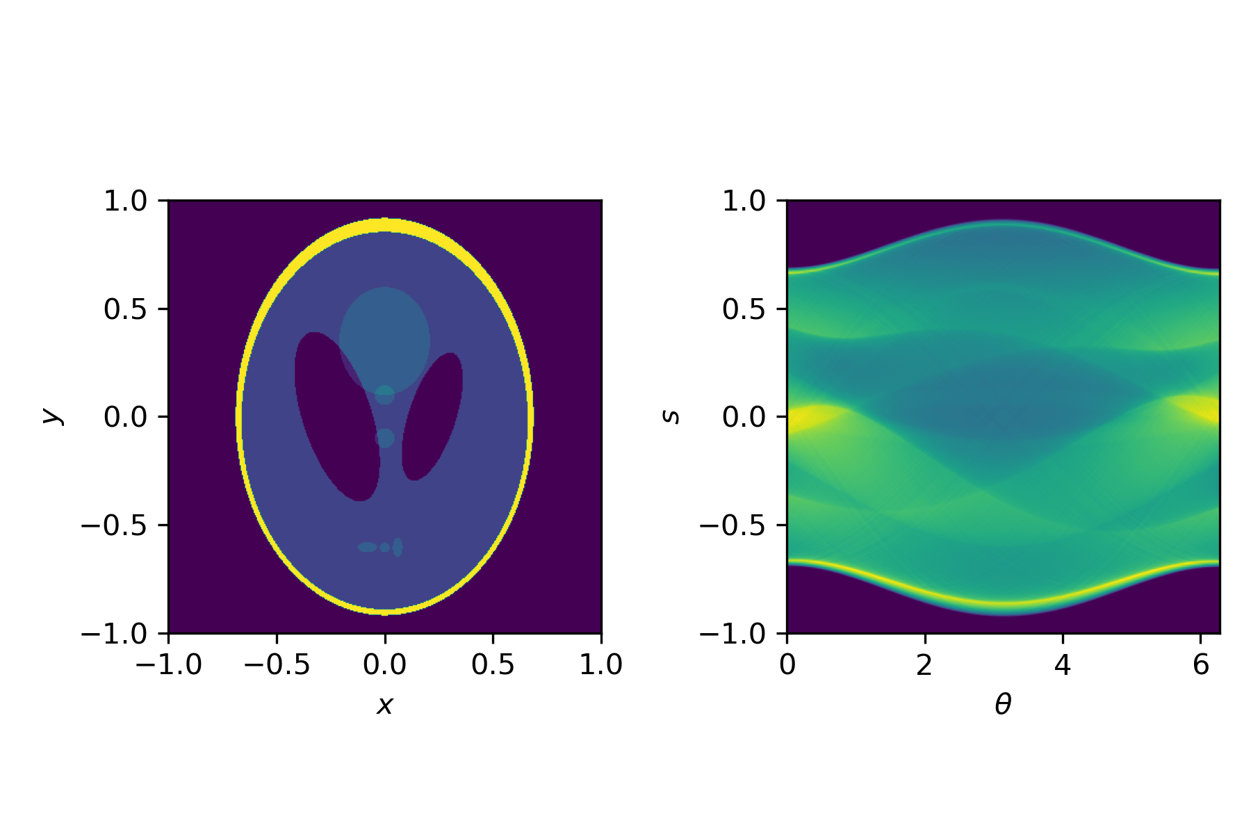
In a CT-scanner, measurements are collected for several rays along different angles, resulting in a sinogram
(Courtesy of Samuli Siltanen)
(Courtesy of Samuli Siltanen)
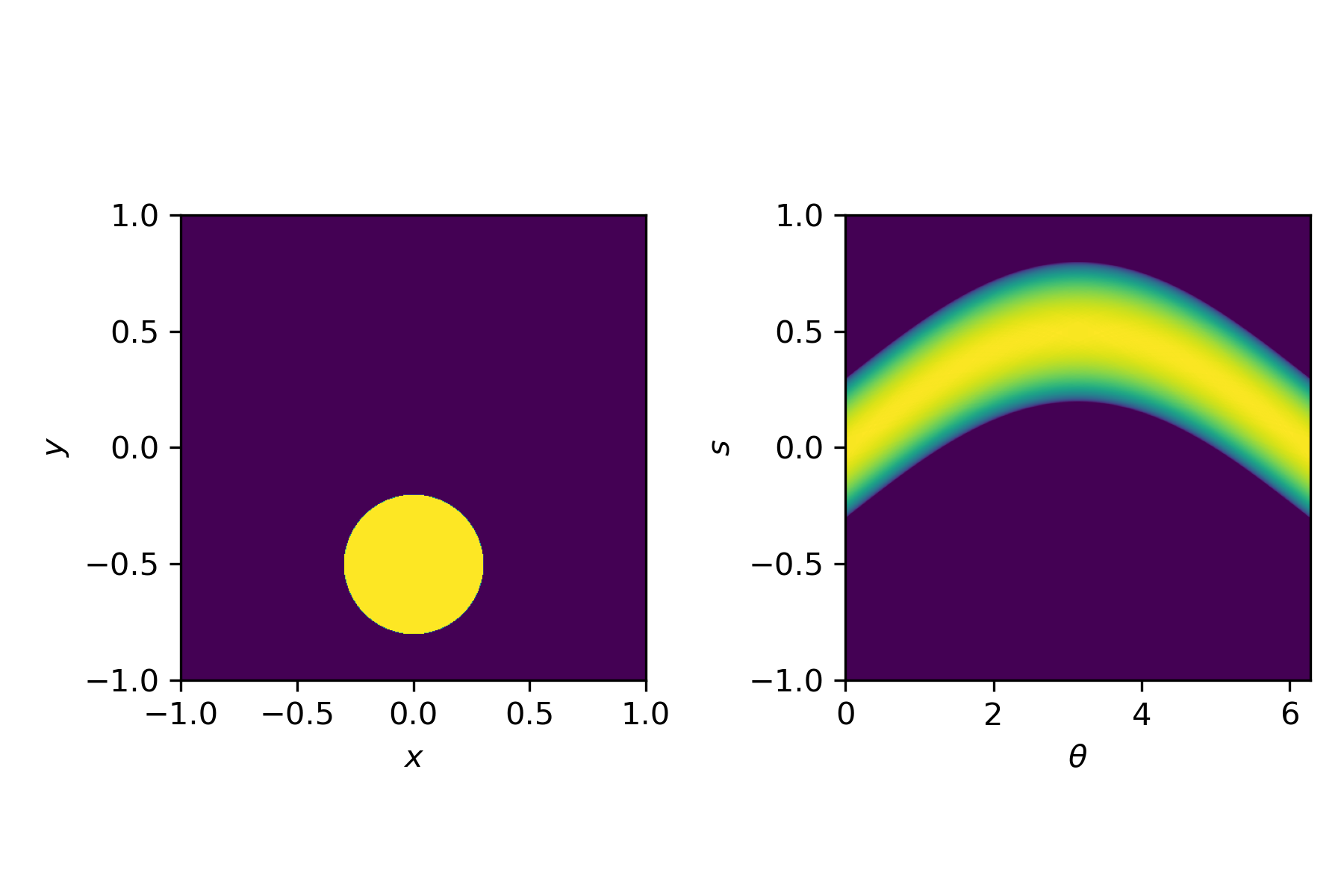
This transformation, from an image $u(x,y)$ to a sinogram $f(\theta,s)$ is described by the Radon transform
$$f(\theta,s) = \int_{-\infty}^\infty u\left(x(s,t), y(s,t)\right) \mathrm{d}t,$$with
$$x(s,t) = t \sin \theta + s \cos \theta, \quad y(s,t) = t\cos\theta - s \sin \theta.$$For simple shapes we can compute the Radon transform by hand. In general, we use a discretised version, for example available in Python via the radon function.
f = radon(u, theta=theta)
Computed Tomography
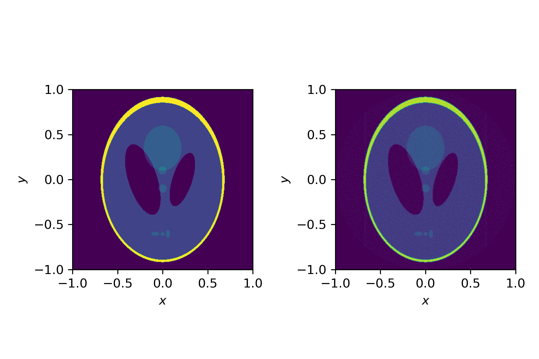
The goal of Computed Tomography is to reconstruct an image $u$ from its sinogram $f$.
- Is the transform invertible?
- What happens if the data are noisy?
- What happens if the data are subsampled?
# settings
nx = 400
na = 400
theta = np.linspace(0., 180., na)
sigma = 1

# phantom
u = shepp_logan_phantom()

# sinogram
f = radon(u, theta=theta)
f_noisy = f + sigma * np.random.randn(nx,na)

# reconstruction
u_fbp = iradon(f_noisy,theta=theta)
Assignments
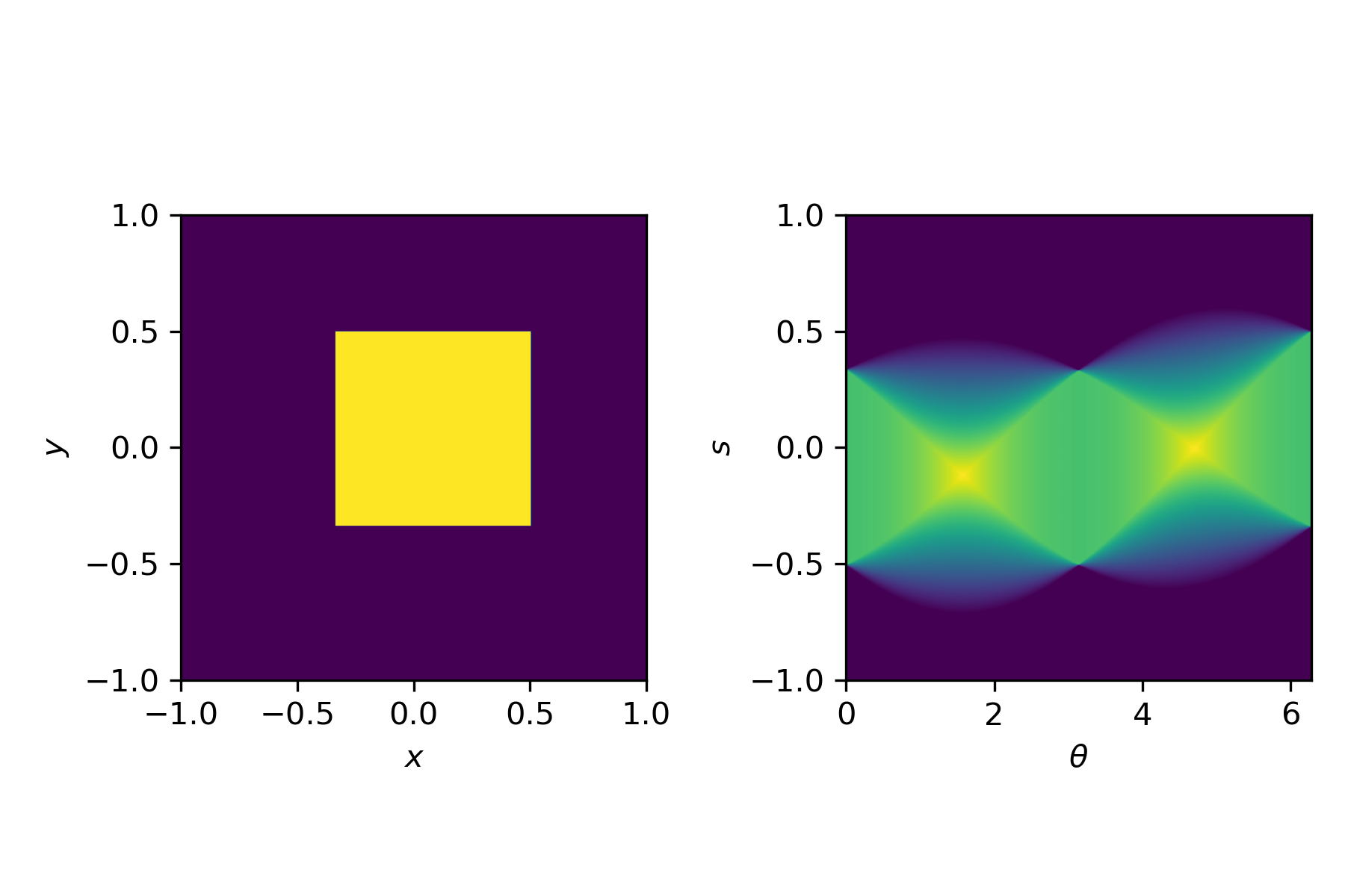
Assignment 1
Compute the exact Radon transform for a uniform square:
$$u(x,y) = \begin{cases}1 & \text{for} & (x,y)\in[-1,1]^2 \\ 0 & \text{otherwise}\end{cases},$$
and compare the result of radon to the exact result.
Assignment 2
Write a function which, for given
thetaandsigmaproduces data for the Shepp-logan phantom, and returns the reconstructed image.Compute the reconstruction error for fixed
theta = np.linspace(0., 180., na)withna = 400for various values ofsigma. Present the results in a graph and table.Compute the reconstruction error for fixed
sigma = 0and varyingna. Present the results in a graph and table.
Draw conclusions about the influence of angular sampling and noise on the reconstruction error.
Some example code can be found on the next slide.
import numpy as np
import matplotlib.pyplot as plt
from skimage.transform import radon, iradon
from skimage.data import shepp_logan_phantom

# settings
nx = 400
na = 400
theta = np.linspace(0., 180., na)
sigma = 1

# phantom
u = shepp_logan_phantom()

# sinogram
f = radon(u, theta=theta)
f_noisy = f + sigma * np.random.randn(nx,na)

# reconstruction
u_fbp = iradon(f_noisy,theta=theta)

# plot
fig,ax = plt.subplots(1,2)

ax[0].imshow(u,extent=(-1,1,1,-1),vmin=0)
ax[0].set_xlabel(r'$x$')
ax[0].set_ylabel(r'$y$')
ax[0].set_aspect(1)

ax[1].imshow(u_fbp,extent=(-1,1,1,-1),vmin=0)
ax[1].set_xlabel(r'$x$')
ax[1].set_ylabel(r'$y$')
ax[1].set_aspect(1)

fig.tight_layout()
/opt/anaconda3/lib/python3.8/site-packages/skimage/transform/radon_transform.py:87: VisibleDeprecationWarning: Creating an ndarray from ragged nested sequences (which is a list-or-tuple of lists-or-tuples-or ndarrays with different lengths or shapes) is deprecated. If you meant to do this, you must specify 'dtype=object' when creating the ndarray
  coords = np.array(np.ogrid[:image.shape[0], :image.shape[1]])
